Tautvidas Sipavičius

We all have stacks of books we bought and never read - information overload pressures us to carefully choose what we devote our scarce attention to. With 2020 coming to a close I thought I’d share several books I’ve enjoyed or found valuable this year - perhaps you fill find a few useful too.

1. High Output Management by Andrew Grove

Andrew Grove (former Intel CEO and Chairman) provides some guidance on how to be effective in a management role by focusing on 4 key areas: business operations, the manager role, scaling beyond a single team, team members as individuals.

The book provided more food for thought for how I fit into my current organization, as well as some ideas I had not considered before, such as the “information gathering and sharing, nudging, decision making” activities managers perform, thinking about processes and bottlenecks as a manufacturer would. If like myself you’ve unintentionally stumbled into a leading or managerial role, “High Output Management” will provide you with a framework for success and deepen your perspective. I would strongly recommend this book.

2. Debugging Teams: Better Productivity through Collaboration by Brian Fitzpatrick and Ben Collins-Sussman

While Robert Martin’s The Clean Coder focuses more on how to “play nice with others” from the individual engineer’s perspective, Fitzpatrick and Sussman extend the same idea to teams (engineering and non-engineering too) and users.

The book builds teamwork on top of 3 pillars: Humility, Respect and Trust, and suggests that most social conflicts arise from lack of one of the components - I’m sure you’ve heard of or (sadly) even experienced horror stories caused by poor company culture or problematic managers/team members. While it’s not a silver bullet, the book provides some guidance for how and why to build team culture, guidance for leaders (lose the ego, providing a safe place for failure), shares several tips for dealing with poisonous people and how to fit within a larger company (e.g. seeking friends, navigating politics).

3. Outliers: The Story of Success by Malcolm Gladwell

The author explores why some people achieve more than others. One of the key points popularized by the book is that it takes about 10 000 hours of practice to master a skill. Of course, success is more than that (e.g. the the book notes opportunity is also a significant contributor to being successful), but as the saying goes “hard work does not guarantee success, but makes it more likely”.

The book altered my mindset for learning new skills. I now look for more (enjoyable) ways to put in the necessary hours of deliberate practice. If we can find enjoyment in practice - we’re more likely to stick with it. And as an added benefit if others view similar practice as work - in the long term we’ll have a competitive edge. E.g. I’m currently going through the FastAI Deep Learning book, and the authors too recommend practicing with domains you’re already an expert in. I find it difficult to internalize some of the datasets (e.g. Kaggle’s Credit Card Fraud), impeding my progress. However, I find it more enjoyable practicing deep learning in building game bots.

On a similar note, a chess streamer GothamChess (IM Levy Rozman) recently talked how in tournament play it’s common to prepare for specific opponents by reviewing their openings and targeting opponent’s less explored lines in an attempt to gain an edge. Being well-rounded is valuable in real world too, so deliberate practice needs to evolve as well.

I find similar ideas resonating in the Masters of Doom book, which described how John Carmack and John Romero built Id Software and its legendary games (such as Doom, Quake, Commander Keen). Both Johns had created tens/hundreds of games and attained mastery even before their paths crossed, and both found sufficiently significant satisfaction in their work to keep pushing their skillsets and the field’s boundary on arduous schedules for years.

4. The Phoenix Project: A Novel about IT, DevOps, and Helping Your Business Win by Gene Kim, Kevin Behr, George Spafford

The book introduces us to the concepts of Lean Manufacturing and the “Three ways” (fast flow of work, enabling fast and constant feedback, continuous learning and experimentation) in the form of a novel, where the story follows Bill - an IT manager tasked with sorting out the mess in the IT department of Parts Unlimited.

I enjoyed this storytelling approach - you get to understand and cringe at the problems (and think “hey, are the authors writing about our organization?”), and then the mentor in the book gradually guides derivation and understanding of solutions, while the main hero stumbles through mistakes and realizations. It provides better context why the devops movement does what it does within a business, shows the problems it solves.

There is a second book - The Unicorn Project, however I found it more difficult to relate to to the point of being distracting, mostly because from what I gathered the characters are portrayed as all-knowing flawless folks at the tippy-top of the field, effortlessly accomplishing all of their tasks and have gotten into the mess only because incompetence of or being undermined by the company, their managers or other teams. Even the mentor from “The Phoenix Project” ended up being a “yes-man”, only praising characters’ ideas rather than actually mentoring.

5. The Design of Everyday Things by Don Norman

The book explores usability design in the real world. While the examples are mostly physical (e.g. how do (or don’t) we know how to open a door?), the underlying principles (discoverability, feedback, affordances) are apt in the software world as well. If you build something for other people to use - this is one of those must-read books.

6. Clean Architecture: A Craftsman’s Guide to Software Structure and Design by Robert Martin

Other Robert Martin’s “Clean” books (clean code, coder) are great, and “Clean architecture” is no different. The book does a deep dive into software architecture, covering basic software design rinciples like SRP, LSP, component design guidelines (e.g. cohesion, coupling) and more architectural topics (layers and boundaries, business rule handling, details).

7. Designing Data-Intensive Applications: The Big Ideas Behind Reliable, Scalable, and Maintainable Systems by Martin Klepmann

The scale of data modern systems utilize continues growing, requiring understanding of how to build scalable and maintainable systems. The book covers 3 major parts: data system fundamentals (reliability, scalability, maintainability, different data storage engines and data evolution over time), distributing data over multiple machines and challenges involved, building systems for deriving data out of existing datasets.

8. Hackers & Painters: Big Ideas from the Computer Age by Paul Graham

You likely already know Paul Graham from YCombinator (the investment company) or Hacker News (the news community for hackers they operate). PG is also an avid writer, you can find his essays here. The book is mostly a compilation of his essays in book form and covers a variety of topics, including fighting spam, how to think about and create wealth, how to think about programming languages and how they shape our work.

9. The Healthy Programmer by Joe Kutner

Software engineers tend to be stereotyped as mostly sedentary, pizza and coke fueled coding machines frequently working late into the night - not the healthiest. The book is especially relevant in today’s COVID world when most of us work from home and barely leave the house, as it provides recommendations on how to set oneself up for a lifelong marathon of staying fit, sharp and healthy, and covers topics like habit building, injury prevention and pain management, nutrition and exercise.

Other interesting mentions

• The Subtle Art of Not Giving a Fuck
• Why We Sleep: Unlocking the Power of Sleep and Dreams
• A Random Walk Down Wall Street: The Time-Tested Strategy for Successful Investing
• The Pleasure of Finding Things Out: The Best Short Works of Richard P. Feynman
• Building Secure and Reliable Systems: Best Practices for Designing, Implementing and Maintaining Systems
• Making Work Visible: Exposing Time Theft to Optimize Work & Flow

I wanted to build a solution to allow dropping off multiple battery-powered sensors (e.g. temperature, humidity, accelerometer) spread out over an area, collecting and processing their data in near real-time. One approach would be to use networking over WiFi, but it is not always available. A while back I wrote about using JY-MCU Bluetooth module to communicate with purpose-built Bluetooth utilities. Now I want to take a step further and set up Bluetooth communication with my own Python app.

The project will look as follows:

• Arduino will collect sensor data, in this case - temperature and humidity data, but it could easily be data from other sensors;
• Arduino will send the sensor data over the JY-MCU Bluetooth module to a Python application we’ll build;
• The Python listener will listen for sensor data and add them to InfluxDB timeseries database;
• Grafana will be used to graph the sensor data from InfluxDB.

1. Arduino setup

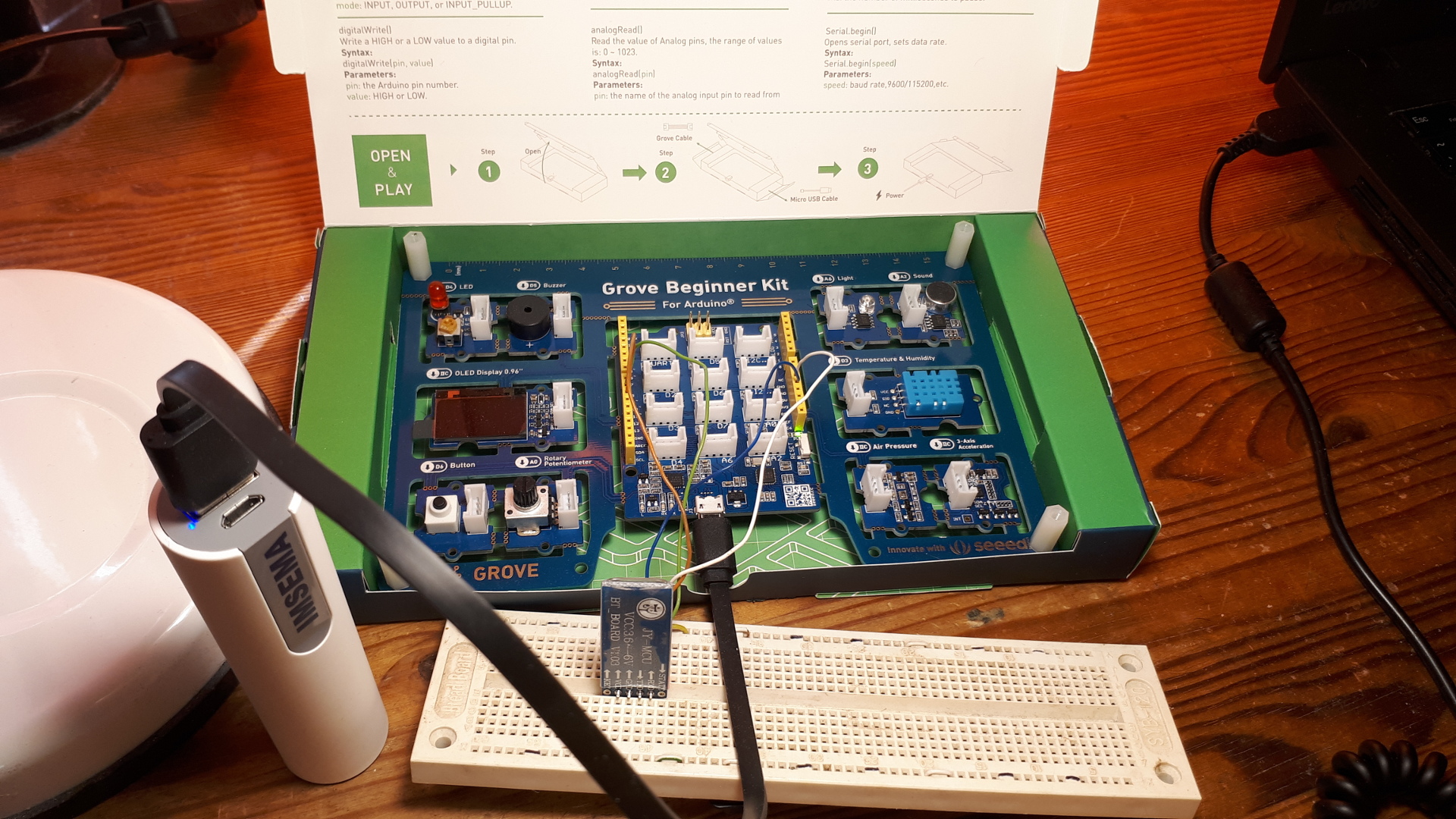
For this proof-of-concept I’ll use the Grove Beginner Kit from Seeed that they graciously sent over. While the kit is intended for beginners and education, it’s also convenient for small scale prototyping, as the kit comes with multiple pre-wired sensors (including the temperature and humidity sensor used here) and uses the modular Grove connector system.

For the bluetooth module, I’ll use the JY-MCU Bluetooth module from DealExtreme, however, DX no longer sell it. I have found a nearly identical version of it as HC-06 on TaydaElectronics: looks like the chips and the model are the same, just screenprinted markings are slightly different.

The temperature/humidity sensor is already connected to Arduino on my kit, unless you break out the sensors out of the PCB. Unfortunately my Bluetooth sensor is not Grove compatible, although with a soldering iron it would be fairly easy to make your own Grove-compatible connector, so I’ll make connections with 4 jumper wires on a breadboard as follows:

• JY-MCU RXD <-> Arduino Pin 9 (MUST SUPPORT PULSE-WIDTH MODULATION)
• JY-MCU TXD <-> Arduino Pin 10 (MUST SUPPORT PULSE-WIDTH MODULATION)
• JY-MCU GND <-> Arduino GND
• JY-MCU VCC <-> Arduino 5V

In the picture above the board is powered by a USB powerbank over a Micro USB connection.

Seeedstudio provide setup instructions and the sample code on how to use the sensor: wiki.

If you’re curious, the library code can be found here: Github. Sensor reads are fairly slow, having to wait for 250ms+, but for this use case it’s good enough.

For the Bluetooth part I’ve used the Arduino IDE built-in SoftwareSerial library.

Third, just for convenience sake, I used ArduinoJson library to send measurements as JSON over bluetooth. While using JSON will waste too much bandwidth on verbose data structures, it will help keep the data processing straightforward, as we’ll need to deal with partial data chunks later on, which would look as follows:

Received chunk b'{'
Received chunk b'"temperat'
Received chunk b'ure":22,"'
Received chunk b'humidity":'
Received chunk b'34}'

Even when trying to read 1kB at a time we get data in chunks. So to get the full record in this case it took 4 reads.

The final code looks as follows:

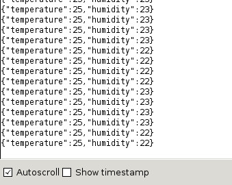
#include <ArduinoJson.h>
#include <SoftwareSerial.h>
#include "DHT.h"

#define DHTPIN 3 // Temperature/Humidity sensor pin
#define DHTTYPE DHT11 // DHT 11
DHT dht(DHTPIN, DHTTYPE);

const int RX_PIN = 10; // Bluetooth RX digital PWM-supporting pin
const int TX_PIN = 9; // Bluetooth TX digital PWM-supporting pin
const int BLUETOOTH_BAUD_RATE = 9600;

SoftwareSerial bluetooth(RX_PIN, TX_PIN);

void setup() {
   dht.begin();
   Serial.begin(9600);
   bluetooth.begin(BLUETOOTH_BAUD_RATE);
}

void loop() {
  StaticJsonDocument<100> doc;

  float measurements[2];
  dht.readTempAndHumidity(measurements);

  doc["humidity"] = measurements[0];
  doc["temperature"] = measurements[1];

  serializeJson(doc, bluetooth);
  serializeJson(doc, Serial);
  Serial.println();
}

No surprises. DHT, SoftwareSerial and ArduinoJson all provide straightforward interfaces to use. This code will read the temperature and humidity sensor data and will write the resulting JSON to Bluetooth and Serial connections.

Serial output looks like this:

2. Python setup

For Bluetooth communication I used Pybluez.

Pybluez can scan for available Bluetooth clients, connect to and communicate with them. However, Pybluez does not provide any utilities to pair with the client, which a StackOverflow comment explains:

PyBluez does not support cross-platform pairing management. This is because some operating systems, like Windows, require super-user level permissions to programatically pair devices. On most operating systems, when PyBluez attempts to connect to the socket using the connect method, the operating system will try to pair (often asking the user for permission).

Inconvenient, so in the end I hardcoded the target address and having to pair the PC with the sensor manually, by using bluetoothctl command from bluez package. Not usable for production, but good enough for a prototype.

Secondly, you see that after receiving every chunk of data we’re trying to parse what we’ve received so far as JSON. This is because data arrives in chunks, and it may take several chunks to receive a valid JSON payload:

Received chunk b'{'
Received chunk b'"temperat'
Received chunk b'ure":22,"'
Received chunk b'humidity":'
Received chunk b'34}'

For InfluxDB I used influxdb-python library, basing the data logging function on their example:

The final code looks like this:

import bluetooth
import json
from influxdb import InfluxDBClient
import datetime

sensor_address = '07:12:05:15:60:07'
socket = bluetooth.BluetoothSocket(bluetooth.RFCOMM)
socket.connect((sensor_address, 1))

influx = InfluxDBClient('localhost', 8086, 'root', 'root', 'example')
influx.create_database('example')

def log_stats(client, sensor_address, stats):
    json_body = [
        {
            "measurement": "sensor_data",
            "tags": {
                "client": sensor_address,
            },
            "time": datetime.datetime.now(datetime.timezone.utc).isoformat(),
            "fields": {
                "temperature": stats['temperature'],
                "humidity": stats['humidity'],
            }
        }
    ]

    client.write_points(json_body)

buffer = ""

while True:
    data = socket.recv(1024)
    buffer += str(data, encoding='ascii')
    try:
        data = json.loads(buffer)
        print("Received chunk", data)
        log_stats(influx, sensor_address, data)
        buffer = ""
    except json.JSONDecodeError as e:
        continue

socket.close()

3. InfluxDB and Grafana

While not necessary, it is convenient to visualize the sensor data, and here I’ve used InfluxDB (a time-series database) and Grafana (a monitoring solution). With one sensor it’s not terribly necessary, but if multiple sensor units were to be used in different locations - graphing the data all in one place makes it much easier to follow and interpret.

I’ve used Docker Compose to run both Grafana and InfluxDB for prototyping purposes. Of course, in a production environment one would want to set up persistence, proper auth, etc.

version: '2.0'
services:
  influx:
    image: influxdb
    ports:
    - "8086:8086"
    environment:
      INFLUXDB_ADMIN_USER: admin
      INFLUXDB_ADMIN_PASSWORD: admin
  grafana:
    image: grafana/grafana
    ports:
    - "3000:3000"
    links:
    - influx

Running docker-compose up will start InfluxDB on port 8086, and Grafana on port 3000.

$ docker-compose ps                                                                                                                                                                                          1 ↵
           Name                     Command           State           Ports         
------------------------------------------------------------------------------------
arduinobluetooth_grafana_1   /run.sh                  Up      0.0.0.0:3000->3000/tcp
arduinobluetooth_influx_1    /entrypoint.sh influxd   Up      0.0.0.0:8086->8086/tcp

I won’t mention all of the setup steps, but some necessary ones:

• Create a new default DB with curl -G http://localhost:8086/query --data-urlencode "q=CREATE DATABASE example"
• Set up InfluxDB connection as a source for Grafana
• Create Grafana dashboards based on sensor data:
  • SELECT max("temperature") FROM "sensor_data" WHERE $timeFilter GROUP BY time(10s) fill(null)
  • SELECT max("humidity") FROM "sensor_data" WHERE $timeFilter GROUP BY time(10s)

4. Results

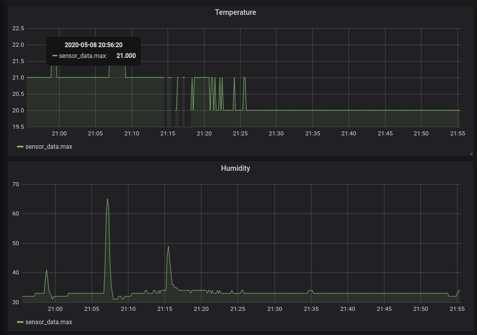
Putting it all together, here’s how the results look like in Grafana. You’ll note that both temperature and humidity are rounded to the nearest integer - this appears to be behavior of the sensor. The three spikes in humidity are from me putting my finger on top of the sensor briefly.

Overall it seems pretty easy to get one device to send data to another device. However, I realize that collecting data from multiple Arduinos would be trickier, requiring to juggle multiple connections, and my JY-MCU Bluetooth module was unable to communicate with multiple Bluetooth clients.

Still, if the Bluetooth module connector was tidied up, it would be fairly easy to break out Arduino and the sensor from the PCB, add a USB powerbank, put it all into an enclosure and have an easily portable data collector.

It was rather convenient to use the Grove Beginner Kit for small scale prototyping like this, as it comes with all sensors already connected in the same PCB, as well as a bunch of sample code to use. If you’d like to pick one up, you can find it here.

When trying to get fit, proper nutrition is essential. Among other things, one needs to watch the calory intake based on TDEE and activity, watch the macronutrients (macro calculator) while ensuring you’re getting sufficient micronutrients. In other words, a giant PITA to plan around.

Commercial tools like EatThisMuch.com are incredibly helpful in meeting the requirements above, adapting to your tastes. Its pricing is not accurate enough for what I can get locally, and it does not have all of the recipes I like. I’m sure I add my recipes to the tool, but why use their complicated solution when I can reinvent my overcomplicated solution?

The approach

With nutrition you get a calory budget. We’ll use 2000 kcal for our example. A common macro split I’ve seen is 34% proteins (4 kcal per 1g), 33% carbohydrates (4 kcal per 1g), 33% fats (9 kcal per 1g), which for our example would result in 170g protein, 165g carbs, 73g fats targets.

I want to minimize the price of the food as well, so our objective is to get as close as we can to the target calories and macros (e.g. within 5-10%) while minimizing the cost - a good objective for a constraint solver to take on. The following implementation will skip micronutrient calculations, just because I don’t have them precalculated for my recipes, but it should be easy to extend the program to support them in the future.

A while back I used Microsoft’s Z3 Theorem Prover’s constraint solving capabilities to solve the PuzLogic puzzle game. It worked well for this use case as well.

The optimization task can be written down as a system of equations:

total_price = meal[0].quantity * meal[0].price + meal[1].quantity * meal[1].price + ... + meal[n].quantity + meal[n].price
total_protein = meal[0].quantity * meal[0].protein + meal[1].quantity * meal[1].protein + ... + meal[n].quantity + meal[n].protein
total_carbs = meal[0].quantity * meal[0].carbs + meal[1].quantity * meal[1].carbs + ... + meal[n].quantity + meal[n].carbs
total_fats = meal[0].quantity * meal[0].fats + meal[1].quantity * meal[1].fats + ... + meal[n].quantity + meal[n].fats
lower_protein_limit <= total_protein <= upper_protein_limit
lower_carbs_limit <= total_carbs <= upper_carbs_limit
lower_fats_limit <= total_fats <= upper_fats_limit
minimize(total_price)

The equations are straightforward to translate for Z3.

Implementation

First we define the targets and some sample meals:

targets = {
    'calories': { 'ideal': 1997, 'lower_limit': 0.8, 'upper_limit': 1.2 },
    'protein': { 'ideal': 170, 'lower_limit': 0.95, 'upper_limit': 1.2 },
    'carbs': { 'ideal': 165, 'lower_limit': 0.9, 'upper_limit': 1.2 },
    'fat': { 'ideal': 73, 'lower_limit': 0.9, 'upper_limit': 1.2 },
    'price': 'minimize',
}

meals = {
    'cottage_cheese': { 'price': 1.4, 'calories': 483.2, 'fat': 11.59, 'carbs': 40.276, 'protein': 55.24, },
    # ... more recipes
    'tortilla_pizza': { 'price': 0.99, 'calories': 510.25, 'fat': 32.04, 'carbs': 26.71, 'protein': 26.66, },
}

Z3 provides convenient objects for Real variables, as well as Sum operations in its Python bindings. We’ll use the optimizer for this program. In its most basic form, we can write the optimizing program as:

from z3 import *

opt = Optimize()
total_price, total_calories, total_protein, total_carbs, total_fat = Reals('total_price total_calories total_protein total_carbs total_fat')
portions_cottage_cheese, portions_tortilla_pizza = Reals('portions_cottage_cheese portions_tortilla_pizza')

# Sum up price, protein, carb and fat totals between our meals
opt.add(total_price == Sum([portions_cottage_cheese*meals['cottage_cheese']['price'], portions_tortilla_pizza*meals['tortilla_pizza']['price']]))
opt.add(total_calories == Sum([portions_cottage_cheese*meals['cottage_cheese']['calories'], portions_tortilla_pizza*meals['tortilla_pizza']['calories']]))
opt.add(total_protein == Sum([portions_cottage_cheese*meals['cottage_cheese']['protein'], portions_tortilla_pizza*meals['tortilla_pizza']['protein']]))
opt.add(total_carbs == Sum([portions_cottage_cheese*meals['cottage_cheese']['carbs'], portions_tortilla_pizza*meals['tortilla_pizza']['carbs']]))
opt.add(total_fat == Sum([portions_cottage_cheese*meals['cottage_cheese']['fat'], portions_tortilla_pizza*meals['tortilla_pizza']['fat']]))

# Add limits that our meals have to sum up to
opt.add(And([
    total_calories >= targets['calories']['ideal'] * targets['calories']['lower_limit'],
    total_calories >= targets['calories']['ideal'] * targets['calories']['upper_limit']]))
opt.add(And([
    total_protein >= targets['protein']['ideal'] * targets['protein']['lower_limit'],
    total_protein >= targets['protein']['ideal'] * targets['protein']['upper_limit']]))
opt.add(And([
    total_carbs >= targets['carbs']['ideal'] * targets['carbs']['lower_limit'],
    total_carbs >= targets['carbs']['ideal'] * targets['carbs']['upper_limit']]))
opt.add(And([
    total_fat >= targets['fat']['ideal'] * targets['fat']['lower_limit'],
    total_fat >= targets['fat']['ideal'] * targets['fat']['upper_limit']]))

# Ensure that portions are non-zero values
opt.add(And([portions_cottage_cheese >= 0, portions_tortilla_pizza >= 0]))

# Let Z3 pick the meal portions while minimizing the price
opt.minimize(total_price)

if opt.check() == sat:
    m = opt.model()
    print(m)

Which outputs:

[portions_cottage_cheese = 150154650/49043707,
 portions_tortilla_pizza = 46250910/49043707,
 total_fat = 657/10,
 total_carbs = 297/2,
 total_protein = 47637960633/245218535,
 total_calories = 192308507415/98087414,
 total_price = 2560049109/490437070]

Or in a more readable format:

[portions_cottage_cheese = 3.061649683210121,
 portions_tortilla_pizza = 0.9430549366914699,
 total_fat = 65.7,
 total_carbs = 148.5,
 total_protein = 194.26737311272169,
 total_calories = 1960.5829083739532,
 total_price = 5.219933943818725]

I had to broaden the upper acceptable range of all of the macros to 1.2x for Z3 to find an acceptable solution with such few possible recipies to choose from, but it did find a satisfactory solution. About 3 portions of cottage cheese and about a portion of tortilla pizza gets us fairly close to the target TDEE and macro requirements.

However, if you run this program multiple times, the result will always be the same. That’s because Z3 only looks for the first satisfactory solution. If we want to instruct Z3 to look for more solutions, we have to invalidate the solutions it already found. Which is fairly easy, just need to change the model displaying part:

variants_to_show = 3
for i in range(variants_to_show):
    if opt.check() != sat:
        break
    if i >= 1:
        print('=' * 80)

    m = opt.model()
    for d in m.decls():
        print(d.name(), m[d].as_decimal(3))

    opt.add(Or([
        portions_cottage_cheese != m[portions_cottage_cheese],
        portions_tortilla_pizza != m[portions_tortilla_pizza]]))

Resulting in:

portions_cottage_cheese 3.061?
portions_tortilla_pizza 0.943?
total_fat 65.7
total_carbs 148.5
total_protein 194.267?
total_calories, 1960.582?
total_price 5.219?
================================================================================
portions_cottage_cheese 2.561?
portions_tortilla_pizza 1.697?
total_fat 84.061?
total_carbs 148.5
total_protein 186.747?
total_calories, 2103.685?
total_price 5.266?
================================================================================
portions_cottage_cheese 3.275?
portions_tortilla_pizza 0.865?
total_fat 65.7
total_carbs 155.034?
total_protein 204
total_calories, 2024.325?
total_price 5.442?

Now we can get Z3 to output a bunch of meal plans for us to choose from.

There are some issues with the code above: it does not scale well with more meals added, the meal portions are calculated in fractions while we’d rather work with full portions, the code could be further cleaned up. But the idea is still there. I ended up with this:

opt = Optimize()

expressions = dict((name, []) for name in targets.keys())
variables = {}

for meal_name, meal in meals.items():
    portions = variables[f'portions_{meal_name}'] = Real(f'portions_{meal_name}')
    opt.add(Or([portions == option for option in [0, 1, 2]])) # Limit to up to 2 full portions per meal

    for target_name in targets.keys():
        expressions[target_name].append(portions * meal[target_name])

expr_to_minimize = None
for name, value in targets.items():
    total = variables[f'total_{name}'] = Real(f'total_{name}')

    if value == 'minimize':
        opt.add(total == Sum(expressions[name]))
        expr_to_minimize = total
    else:
        opt.add(total == Sum(expressions[name]))
        opt.add(total >= value['ideal'] * value['lower_limit'])
        opt.add(total <= value['ideal'] * value['upper_limit'])

optimized = opt.minimize(expr_to_minimize)
variants_to_show = 5
for i in range(variants_to_show):
    if opt.check() != sat:
        break
    if i >= 1:
        print('=' * 80)

    m = opt.model()
    for name, variable in variables.items():
        if name.startswith('portions_') and m[variable] == 0:
            continue

        if m[variable].is_real():
            print(name, m[variable].as_decimal(3))
        elif m[variable].is_int():
            print(name, m[variable].as_long())
        else:
            print(name, m[variable])

    # Ignore already found variants
    opt.add(Or([variable != m[variable] for name, variable in variables.items() if name.startswith('portions_')]))

Results

With a bigger set of recipes to choose from, Z3 came up with the following meal plans:

portions_peanuts 2
portions_protein_pancakes 2
portions_chicken_quesadilla_w_cheese 1
total_calories 1994.24
total_protein 169.76
total_carbs 164.76
total_fat 77
total_price 3
================================================================================
portions_peanuts 1
portions_protein_pancakes 2
portions_pulled_pork_quesadilla 2
total_calories 2088.18
total_protein 168.39
total_carbs 180.74
total_fat 79.38
total_price 3.11
================================================================================
portions_chicken_pilaf 1
portions_peanuts 2
portions_protein_pancakes 1
portions_chicken_quesadilla_w_cheese 1
total_calories 2051.22
total_protein 168.23
total_carbs 172.24
total_fat 78.6
total_price 3.46
================================================================================
portions_chicken_quesadilla 1
portions_protein_pancakes 2
portions_tortilla_pizza 1
total_calories 1917.45
total_protein 162.78
total_carbs 171.85
total_fat 66.5
total_price 3.61
================================================================================
portions_almonds 1
portions_peanuts 1
portions_protein_pancakes 2
portions_chicken_quesadilla_w_cheese 1
total_calories 1979.74
total_protein 166.91
total_carbs 162.91
total_fat 80
total_price 3.77

And with a bigger bank of recipes it beats me having to plan it all out. Now I can let it generate hundreds of plans for me to choose from, and they’ll all be composed of recipes I like and based on prices at my grocery store. Granted, some of the suggestions are not great: not doable for time reasons or personal tastes, lack of micronutrients (e.g. the plans should definitely include more veggies), but it’s a decent starting point. With a selection of better recipes the meal plans would be better too.

You can play around with the full implementation on Google’s Colaboratory.

I’ve recently been toying with Sonic-Pi - a code based music creation tool created by Sam Aaron. It’s written in Ruby on top of SuperCollider and is designed to handle timing, threading and synchronization specifically for music creation.

An older music creation library Overtone, authored by Sam Aaron as well, included the famous THX Surround Test sound simulation example: Code. This inspired to try replicate a different interesting sound - the Shepard tone - using Sonic-Pi.

Shepard tone

Shepard tone has an interesting property, in that it feels like it is always increasing in pitch. The effect can be achieved by playing multiple tones with an increasing pitch at the same time, one octave (or a double in frequency) apart. Each tone starts at a low frequency and fades-in in volume, gradually increasing in pitch, and fades-out upon reaching a high pitch as another tone takes its place.

The spectrum diagram by Grin (CC BY-SA) illustrates the construction well. Note that the red lines are going up over time in pitch, the thickness of a line - volume - increases as it fades in at a low pitch, and decreases as it fades out at a high pitch.

Constructing the tone

Sonic-Pi has a neat sliding mechanism, allowing us to start from one pitch and slide it up to another pitch:

synth = play note(:C3), note_slide: 1
control synth, note: note(:C4)
sleep 1

Here it starts by playing a C3 note using a sine wave synthesizer, and slides it up by one octave to a C4 note over one beat (or 1 second at a 60bpm default tempo):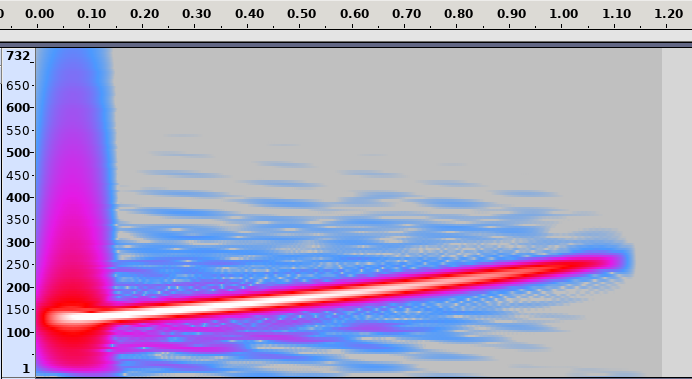

Extending this example would allow us to build a tone with an increasing pitch, but it plays always at max volume.

The second building block is volume control. The tone needs to fade in at the beginning, reach a maximum volume, and fade out at some high pitch. Sonic-Pi provides an ADSR envelope generator we can use for this purpose.

ADSR stands for Attack, Decay, Sustain, Release and describes how sound changes over time, or in this case - its volume.

Abdull’s diagram on Wikipedia illustrates the use well. Imagine pressing a piano key. If you press it quickly and forcefully, it reaches the full volume quickly (the Attack stage), then decays to some sustainable volume (the Decay stage) that is sustained for a while (the Sustain stage), after you release the key - the sound quickly diminishes to zero.

This mechanism can be conveniently used to build the fade-in and fade-out of our sine wave:

synth = play note(:C3), note_slide: 5, attack: 1, decay: 0, sustain: 3, release: 1
control synth, note: note(:C4)
sleep 5

I’ve increased the duration of the wave to 5 beats to illustrate the example. But following the ADSR envelope diagram above, the sound will go from 0 to 100% volume in 1 beat. Decay is 0, so we can ignore it. It will stay at maximum volume for 3 beats, and then go from 100% to 0% volume in 1 beat. All the while the pitch of the sound is increasing from C3 to C4.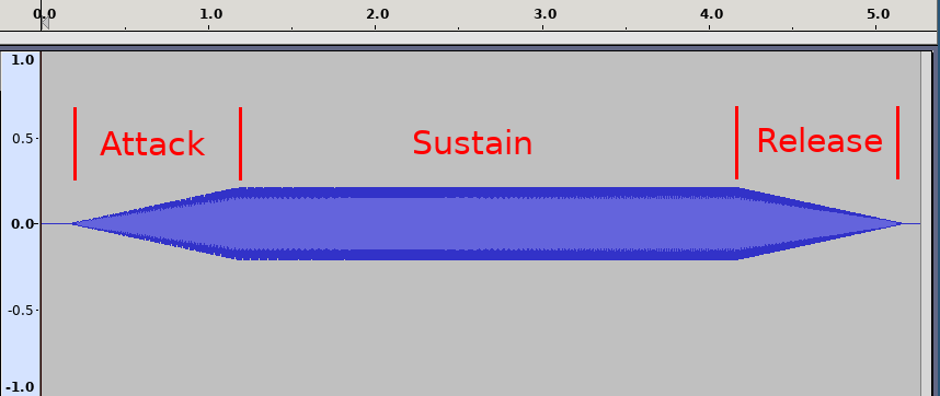

The last building block is to play multiple tones at the same time. Sonic-Pi handles threading for us very well, and in Sonic-Pi commands are executed in parallel. E.g. if we try to play two tones at once, the code would look as follows:

play note(:C3)
play note(:C4)
sleep 1

Both notes C3 and C4 would be played at the exact same time for 1 second.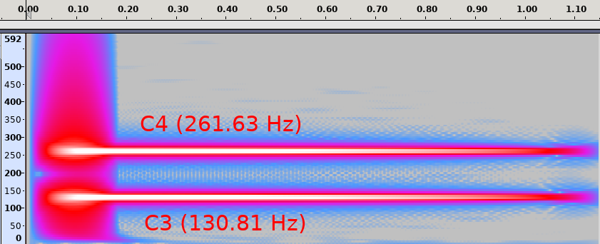

In a similar vain, the idea would be to sequentially start multiple waves we created above in independent threads, sleeping for a bit to start another wave just as others have reached octaves. This can be done roughly as follows:

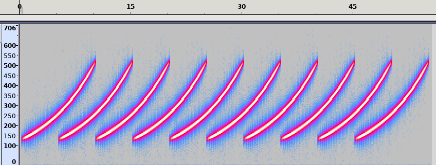
total_waves = 10
total_waves.times do
  in_thread do
    synth = play note(:C3), note_slide: 10, attack: 1, decay: 0, sustain: 8, release: 1
    control synth, note: note(:C5)
    sleep 10
  end
  sleep 5
end

I’ve further increased the duration of a single sine wave to 10 seconds, and the pitch to rise from C3 to C5, or two octaves. The code above will play 10 such sine waves, start of each separated by 5 beats. That way:

• At second 0 the first sine wave will start playing at C3, fading-in in volume
• At second 5, the first sine wave would have reached C4 note at full volume, then a second wave would start playing a C3 note also fading-in in volume;
• At second 10, the first wave would have reached C5 and would’ve finished fading out. The second wave would have reaced C4 note, and a third wave would’ve started playing a C3 note, and so on.

All 3 construction components put together, cleaned up and synchronized using the cue/sync resulted in the following final snippet:

starting_note = note(:C2)
total_octaves = 4
octave_duration = 10
total_waves = 20
wave_duration = octave_duration * total_octaves
fade_in_out_duration = wave_duration * 0.2

target_notes = octs(starting_note, total_octaves + 1).drop(1)

in_thread do
  total_waves.times do
    sync :new_octave
    in_thread do
      with_synth :sine do
        instrument = play starting_note,
          note_slide: octave_duration,
          attack: fade_in_out_duration, release: fade_in_out_duration,
          decay: 0, sustain: (wave_duration - 2 * fade_in_out_duration)

        total_octaves.times { |octave|
          cue :new_octave
          control instrument, note: target_notes[octave]
          sleep octave_duration
        }
      end
    end
    sleep octave_duration
  end
end

cue :new_octave

And the end result would sound like this:

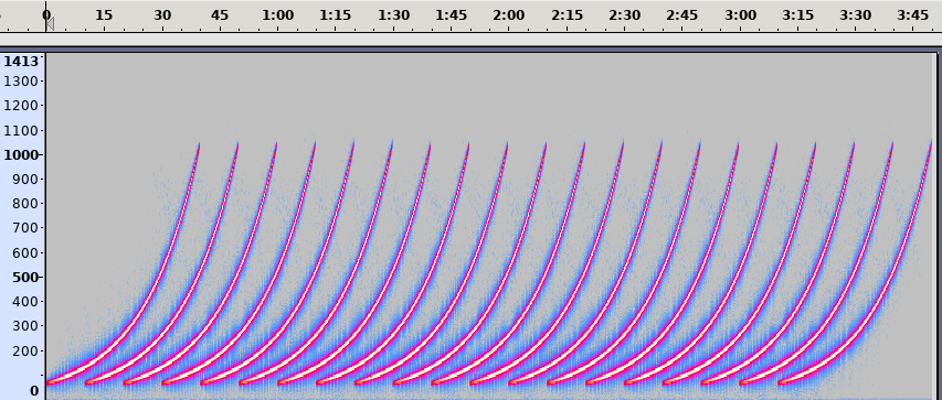
Overall I’m rather impressed by Sonic-Pi’s ability to handle threading, synchronization and sliding. It resulted in a fairly short piece of code, and could likely be made smaller still by replacing the octave-target loop with a single control call to linearly slide the starting note to the highest note the sine wave is supposed to reach.

TL;DR: Here is some resulting gameplay from this Dueling Double Deep Q-learning network based bot:

For a while I wanted to explore Reinforcement learning, and this time I’ve done so by building a Q-Learning based bot for the Bubble Shooter game - an Adobe Flash based game running in the browser.

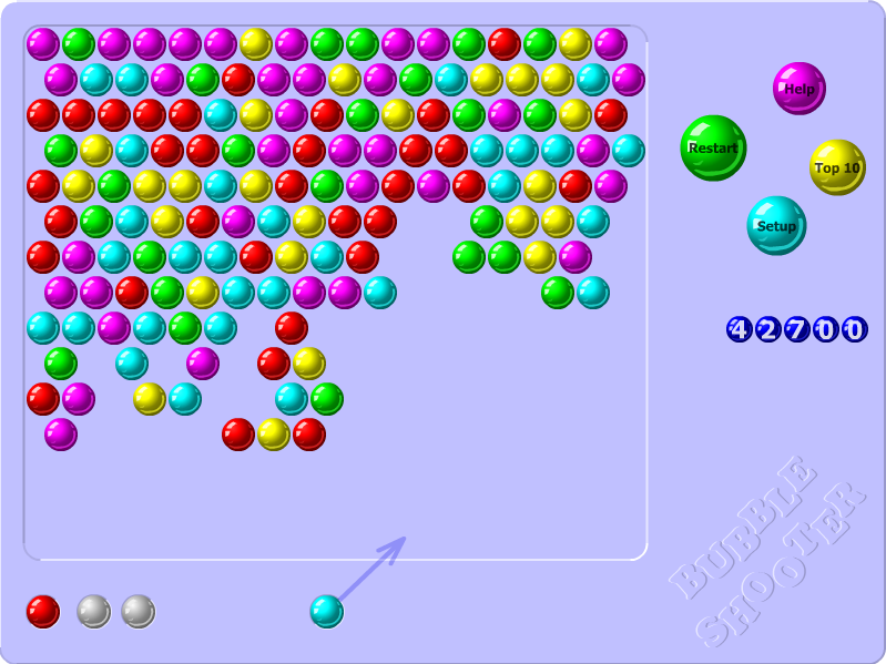
The game works as follows: the game board contains bubbles of 6 different colors. Shooting a connected group of same colored bubbles with 3 or more bubbles in it destroys all of them. The goal of the game is to destroy all bubbles on the board.

I chose the game for simplicity of its UIs and 1-click gameplay, which was reasonably straightforward to automate.

What is Q-Learning?

You can learn about it in more detail by reading this Wikipedia article or watching this Siraj Raval’s explanatory video.

But in short, in Q-Learning given a state the agent tries to evaluate how good it is to take an action. The “Q” (or “Quality”) value depends on the reward the agent expects to get by taking such action, as well as in any future states.

E.g. maybe the agent shoots a bubble in one place and doesn’t destroy any bubbles - probably not a great move. Perhaps it shoots a bubble and manages to destroy 10 other bubbles - better! Or perhaps it does not destroy any bubbles on the first shot, but this enables the agent to destroy 20 bubbles with the second shot and win the game.

The agent chooses its moves by calculating Q-values for every possible action, and choosing the one with the largest Q-value - the move it thinks will provide it with the most reward.

For simple cases with few unique game states one can get away with a table of Q-values, but state of the art architectures switched to using Deep Neural Networks to learn and predict the Q-values.

Dueling Double Q Network architecture

The simplest case is a Deep Q Network - a single deep neural net that attempts to predict the Q-value of every step. But apparently it is prone to overestimation, resulting in the network thinking the moves are better than they really are.

An improvement of that was Double Q Network (Arxiv paper: Deep Reinforcement Learning with Double Q-learning), which has two neural networks: an online one and a target one. The online network gets actively trained, while the target one doesn’t, so the target network “lags behind” in its Q-value evaluations. The key is that the online network gets to pick the action, while the target network performs the evaluation of the action. The target network gets updated every so often by copying the Neural Network weights over from the online network.

A further improvement still was a Dueling Q network (Arxiv paper: Dueling Network Architectures for Deep Reinforcement Learning). The idea here is that it splits out the network into 2 streams: advantage and value, results of which are later combined into Q-values. This allows the network to learn which states are valuable without having to learn the effect of every action in the state, allowing it to generalize better.

In the end I’ve ended up combining all of the techniques above into the following network:

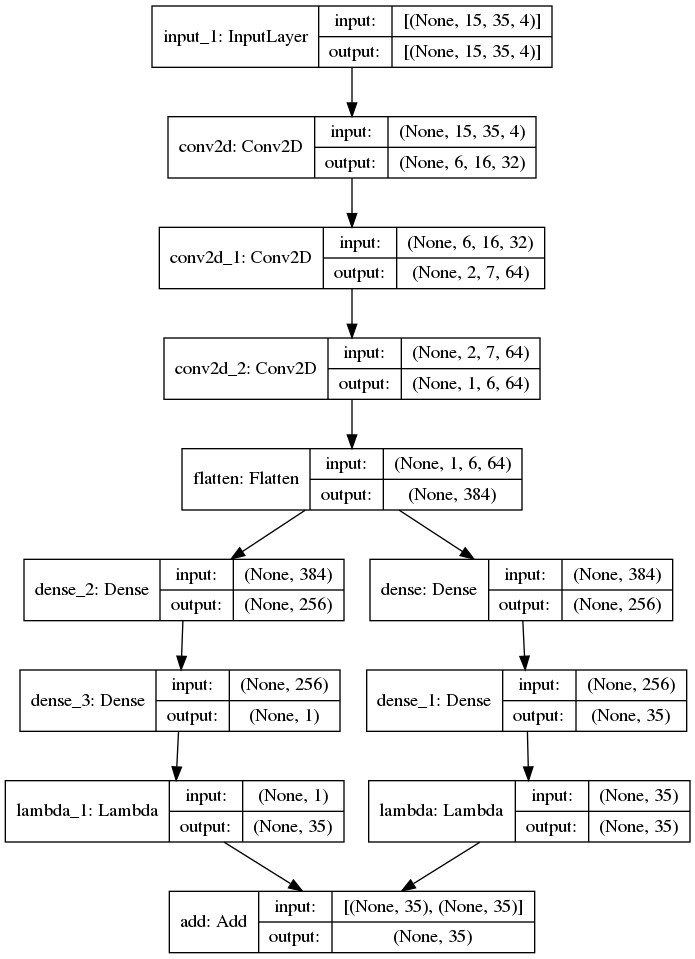
It’s based on the architecture mentioned in one of the papers: several convolutional layers followed by several fully connected layers.

Game states and rewards

DeepMind were able to get their model successfully playing 2600 Atari games just by taking game screenshots as an input to the neural net, but for me the network simply failed to learn anything. Well, aside from successfully ending the game in the fewest number of steps.

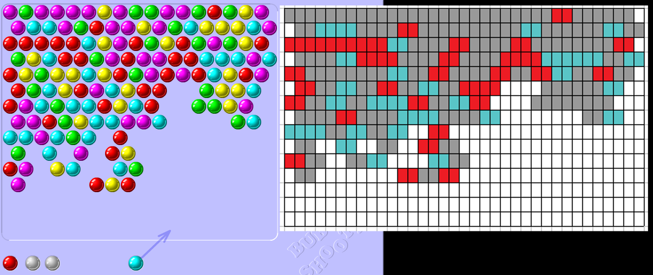
So I ended up using Computer Vision to parse the game board into a 35x15 matrix. 35 ball halves fit horizontally, and 15 balls fit vertically into a game board, so every cell in a matrix represents a half-ball horizontally and a full-ball vertically.

What the current agent actually sees though are 4 different snapshots of the game board:

• Positions of half-balls that match the current ball’s color
• Positions of half-balls that don’t match the current ball’s color
• Positions of half-balls that match the next ball’s color
• Positions of half-balls that don’t match the next ball’s color

The idea was to start with at least learning the game for the current and the following ball colors to simplify the rules. I tried having layers for balls of every color, but wasn’t able to make it work yet.

For rewards, I’ve settled on two: destroying more than one ball gives a reward of 1, every other action gives a reward of 0. Otherwise I found that Q-values gradually grow to infinity.

For possible actions, the game board is 500x500 px in dimensions, meaning that there are 250000 possible actions for every state, that means lots of computations. To simplify, I’ve narrowed the action space down to 35 different actions, all oriented in a single horizontal line ~100px from the bottom of the game board.

This makes some further shots impossible due to lack of accuracy, but seems to be good enough to start with.

Prioritized experience replay

The first option is to start with no replay at all. The agent could take a step and learn from it only once. But it is a poor option, as important experiences may be forgotten, and adjacent states correlate with each other.

An improvement over it was to keep some recent experiences (e.g. 1 million experiences), and to train the neural network based on a randomly sampled batch of experiences. This allows to avoid correlation of adjacent states, but important experiences may still end up being revisited rarely.

A further improvement over that is to keep a buffer of prioritized experiences. The experiences are prioritized based on the Q-value error (difference of predicted Q-value and actual Q-value), and training the neural network by sampling batches from different ranges of errors. That way more error-prone but rarely occurring states have a better chance of being retrained upon.

I ended up using Jaromiru’s (based on this article) reference implementation of Prioritized Experience Replay (SumTree, Memory).

An experience is a tuple of:

• The current state
• The action taken
• The reward received
• The next resulting state
• Whether the episode is “done”

Training in parallel

Originally I’ve started with just a single instance of the game for training, but Machine Learning really shines with lots and lots of data (millions, billions of samples - the more the better), so at 2-5 seconds per step it just took too long to get any substantial amount of training done.

So I used Selenium+Firefox and Python’s multiprocessing module to run 24 isolated game instances at once, allowing it to top out at about 4 steps/second. Even at the low number of instances it’s quite CPU-heavy and makes my poor Ryzen 2700x struggle, making the games run slower.

You can find an explanation on how it was done in my last post, or find the code on Github.

Results

The most successful hyperparameters so far were:

• Exploration probability (epsilon): 0.99
• Minimum exploration probability: 0.1 and gradually reducing to 0.01 with every training session
• Exploration probability decay every episode: 0.999 gradually reducing to 0.9 with every training session
• Gamma: 0.9
• Learning rate: 0.00025
• Replay frequency: every 4 steps
• Target network update frequency: every 1000 steps
• Memory epsilon: 0.01
• Memory alpha: 0.6
• Experience memory buffer: 20000 experiences
• Batch size: 32

In total the model was trained about 6 different times for 200-300k steps - for ~24h each time.

During training the model on average takes ~40 steps (~70 max), and is able to destroy at least 2 bubbles ~19 times in an episode (~39 max).

The resulting gameplay is not terribly impressive, the agent is not taking some clear shots when there’s nothing better to do. Its knowledge also seems to be concentrated close to the starting state - it’s not doing well with empty spaces closer to the top or bottom of the board. But it is playing the game to some extent, and if the game’s RNG is favorable - it may even go pretty far.

As a next step I might try different network architectures and hyperparameters, to speed things up pretrained offline on the bank of experiences acquired from this model’s gameplay.

If you’re interested in the code, you can find it on Github.