Tautvidas Sipavičius

In the previous post we looked into applying basic pattern matching with OpenCV to build a basic bot to play Burrito Bison browser game. However, there was very little game logic involved: it watched and waited for powerups to fill up, using them once filled up. Everything else was related to keeping the game flow going by dealing with menus.

In this post (or next few posts) let’s take a look at a slightly different game: Puzlogic. Puzlogic is somewhat similar to sudoku and comes with 15 different levels. The goal of the game is to place a set of given numbers into a grid where some cells are pre-filled with other numbers. The catch is that duplicates are not allowed in any column or row, and in some cases extra constraints can be applied, e.g. that numbers on a given column or row would add up to a specific sum.

I would recommend you to play the game for several rounds to familiarize with it.

But I think Puzlogic is a convenient problem to explore several approaches on:

1. More elaborate computer vision approaches to understand the grid, e.g. recognition of digits, identifying different elements (irregularly spaced grid, set of given numbers, sum constraints)
2. Solve the puzzle using Python, e.g. using a bruteforce approach, or using a theorem prover like Z3.
3. Lastly, combine the two components above and use the a mouse controller like Pynput to tie it all together.

In this first post let’s start with the puzzle solver first, tackling CV and controls portion in later posts.

Planning

Again, at first I’d recommend completing a first few puzzles manually to learn how the game works. But here are my first impressions:

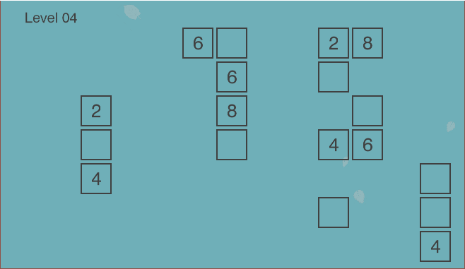
The game board is in the form of the grid. However, not every location in the grid is a valid cell - there may be spaces around valid cells. Some valid cells have pre-filled numbers in them which cannot be overwritten, while empty cells are intended for the player-controlled pieces.

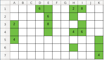
Since it is a grid, we can think about it as an NxM matrix, where N and M are distances between furthest horizontal and vertical valid cells. However, because most cells may not be valid, it would be a waste of space to represent it as a two-dimensional array. Instead it can be represented as a Sparse matrix using a coordinate list, where each cell is represented as (x_coordinate, y_coordinate, value) triplet. So the full grid would be represented as: [(x_0, y_0, value_0), (x_1, y_1, value_1), ... (x_n, y_n, value_n)].

Secondly, the numbers player has to use (we’ll call them “pieces”) are displayed near the bottom of the window in another grid, which means coordinates will be important later when moving the pieces to the game board. That can be represented as a simple list of integers: [piece_0, piece_1, ..., piece_n]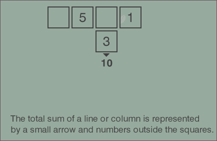

Third, if you play a few more rounds of the game, you’ll see how sum constraints are displayed. They can be applied to any row or any column. We can represent the constraint with another triplet: (index, 'column', target_sum) or (index, 'row', target_sum). The list of constraints then would be represented as: [(index_0, dimension_0, target_0), ..., (index_n, dimension_n, target_n)].

So we have our three parameters: grid, pieces and constraints.

And lastly, how would a solution be represented? The game is won once all the game pieces are moved to the game board, the game board is valid and all constraints are satisfied. So we could represent the solution as a list of moves, where a move is a triplet (x, y, piece), denoting on which coordinates each piece should be placed.

The number of pieces is low, the size of the game board is also small, so we can use a brute force depth-first search to find at least one solution.

Implementation

For pseudocode of the algorithm, I think a pattern I’ve seen used during Martin Odersky’s Scala classes works well here:

1. Generate all possible moves for the given position;
2. Filter the list of all moves leaving only the legal moves;
3. Recursively repeat from step 1 with the new game state.
4. If the solution is found - recursively return it through the execution tree, if not - allow the depth-first search to continue until the whole search space is exhausted.

Let’s start at the top with solution() and fill in the blanks:

    def solve(self, board, pieces, constraints=[]):
        if len(pieces) == 0:
            return []

        for (move, new_board, new_pieces, new_constraints) in self.legal_moves(board, pieces, constraints):
            solution = self.solve(new_board, new_pieces, new_constraints)
            if solution != False:
                return [move] + solution

        return False

This is following the exact same pattern as outlined above: generates new states for each of the legal moves, and continues exploring the new legal states one by one. If the solution has been found - the current move would be added to the solution. If not - the search continues until exhaustion.

legal_moves is missing, so let’s implement it next. What it has to do is for each piece in the pieces list generate a new state (board, remaining pieces) as if we made the move. Constraints don’t really change, so we can return the same argument. As per above, it would need to return the quadruplet: (move, new_board, new_pieces, constraints).

    def legal_moves(self, board, pieces, constraints):
        return (move for move in self.all_moves(board, pieces, constraints) if self.is_legal(move[1], constraints))

Here a generator expression is used to avoid having to store all possible moves in memory at once as search space is explored at each recursion depth. Instead the first matching value will be generated, the generator will return, search will continue in the deeper search level.

Subsequently, all_moves() can be defined as:

    def all_moves(self, board, pieces, constraints):
        """ Attempt to put one of available pieces into the available spaces on the board """
        free_cells = [(c[0], c[1]) for c in board if c[2] == 0]
        return (
            ((row, column, piece), new_board, new_pieces, constraints)
            for (row, column) in free_cells
            for piece in pieces
            for (new_board, new_pieces, new_constraints) in [self.perform_move((row, column, piece), board, pieces, constraints)]
        )

All it does is it attempts to place one of the available pieces into one of the free cells on the board.

When making a move, the selected piece is no longer available in the pieces list for further use. Instead it’s placed into the board matrix at given coordinates, making it permanent for deeper recursion to work with.

    def perform_move(self, move, board, pieces, constraints):
        """ Moves the given piece to the location on the board """
        new_pieces = pieces.copy()
        new_pieces.remove(move[2])

        new_board = board.copy()
        new_board.remove((move[0], move[1], 0))
        new_board.append(move)

        return new_board, new_pieces, constraints

Next let’s take care of is_legal(), which evaluates whether a given board is legal:

    def is_legal(self, board, constraints):
        """
        Is the board legal.
        - Rows and columns contain no duplicates
        - If there are constraints and all cells are filled in a given column - the sum of the column does not exceed the constraint
        - If all cells are filled in - constraint matches
        """

        lines = self.rows(board) + self.columns(board)

        no_duplicates = all(self.all_unique(self.filled_cells(line)) for line in lines)
        satisfies_constraints = all(self.satisfies_constraint(board, c) for c in constraints)

        return no_duplicates and satisfies_constraints

The uniqueness constraint in rows and columns:

    def all_unique(self, line):
        return len(line) == len(set(line))

    def rows(self, board):
        return self._lines(board, 0)

    def columns(self, board):
        return self._lines(board, 1)

    def _lines(self, board, dimension=0):
        discriminator = lambda c: c[dimension]
        cells = sorted(board, key=discriminator)
        groups = itertools.groupby(cells, key=discriminator)
        return [[c[2] for c in group] for index, group in groups]

    def filled_cells(self, line):
        return [x for x in line if x != 0]

The end goal of the summing constraint is to make sure that once all cells are filled in a line that the target sum is reached. However, in order for us to perform the search there will be times when some cells are not filled in. In such cases we’ll consider the constraint satisfied only if the sum of a line is lower than the target sum - there’s no point in continuing the search if we already blew over the limit.

    def satisfies_constraint(self, board, constraint):
        (dimension, element, target_sum) = constraint
        line = self._lines(board, dimension)[element]
        line_sum = sum(line)
        return (
            (line_sum == target_sum and self.all_cells_filled(line))
            or
            (line_sum < target_sum)
        )

That’s it!

And that’s it! We should have a working solver for the puzzle. Of course, having tests would be good to make sure it actually works and keeps on working, and I’ve already done that in the project’s repo.

Now we can test it out with the first level:

solver = Solver()
board = [
    (0, 1, 1),
    (1, 0, 0),
    (1, 1, 0),
    (2, 0, 2)
]
pieces = [1, 2]

moves = list(solver.solve(board, pieces, []))
print(moves)

# > [(1, 0, 1), (1, 1, 2)]

Or the third level:

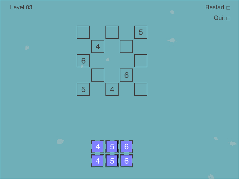
solver = Solver()
board = [
    (0, 0, 0),
    (0, 2, 0),
    (0, 4, 5),
    (1, 1, 4),
    (1, 3, 0),
    (2, 0, 6),
    (2, 4, 0),
    (3, 1, 0),
    (3, 3, 6),
    (4, 0, 5),
    (4, 2, 4),
    (4, 4, 0),
]
pieces = [4, 5, 6, 4, 5, 6]

moves = list(solver.solve(board, pieces, []))
print(moves)

# > [(0, 0, 4), (0, 2, 6), (1, 3, 5), (2, 4, 4), (3, 1, 5), (4, 4, 6)]

Looks like it works! While this is not a very elegant approach, a brute force approach with small numbers still seems sufficient, which is great for the toy application. In the next post I’ll start looking into the computer vision part.

If you’d like to see the full code of the solver, you can find it on the project’s Github repo: puzbot - solver.py.

Let’s Encrypt has taken certificate business by storm, issuing over 50 million active certificates (stats). It is free and easy way to start using HTTPS on your website to secure the traffic.

One slight inconvenience is that certificates themselves are fairly short lived (only 90 days) and require renewals. Luckily, there are automated tools like Certbot which help you handle renewals. If you have it set up just right, you can create a cron job and it will continuously renew the cert for you. E.g. I use geerlingguy.certbot Ansible role for it.

However, recently I noticed that the renewal started failing with the following error message:

Attempting to renew cert (hermes.tautvidas.lt) from /etc/letsencrypt/renewal/hermes.tautvidas.lt.conf produced an unexpected error: Failed authorization procedure. hermes.tautvidas.lt (tls-sni-01):
+urn:acme:error:tls :: The server experienced a TLS error during domain verification :: remote error: tls: handshake failure. Skipping.
All renewal attempts failed. The following certs could not be renewed:
  /etc/letsencrypt/live/hermes.tautvidas.lt/fullchain.pem (failure)
1 renew failure(s), 0 parse failure(s)

As per this ticket, Let’s Encrypt will try to match the requester server’s IP address with given domain’s DNS A record IP:

To fix these errors, please make sure that your domain name was
entered correctly and the DNS A/AAAA record(s) for that domain
contain(s) the right IP address. Additionally, please check that
your computer has a publicly routable IP address and that no
firewalls are preventing the server from communicating with the
client. If you’re using the webroot plugin, you should also verify
that you are serving files from the webroot path you provided.

However, if you have CloudFlare enabled for that domain and you have it configured to run in HTTP Proxy mode - CloudFlare might be interfering. That is because of how CloudFlare CDN works: visitors will connect to CloudFlare’s servers, and if CF can - it will return them the requested resource without ever passing the request to your servers, if it cannot - it might request your server for that resource. But whatever happens, the visitor will see that it is connecting to CloudFlare’s servers - not yours!

So if you do have CloudFlare’s HTTP Proxy enabled, consider disabling the Proxy mode for that particular (sub)domain:

You should be able to renew the certificate after doing so.

However, if you cannot disable CloudFlare’s HTTP proxy for your domain, consider using CloudFlare’s Origin Certificate to encrypt communication between your server and CloudFlare, and use CloudFlare’s Universal SSL between CloudFlare and your visitors.

Last time I participated in the Practice round of Google Code Jam 2018. It was a fun experience, so on 2018-04-07 I went for the Qualification round.

While practice round took about 7 hours to complete, the qualification round topped that requiring about 10h of work. As previously, there 4 problems with one visible and one hidden result each. I managed to correctly complete 1/2 tests for the first three, and then 2/2 tests for the fourth one for a total of 55/100 points. Bummer!

But, here’s how I approached the problems.

1. Saving the universe again

Problem description.

In short, a killer robot is executing a program, which consists of 2 instructions. C charges the weapon, doubling the damage, S shoots the weapon. Hero can swap two adjacent instructions, but want to do so as few times as possible. What is the minimum number of such changes have to be made so that the robot doesn’t do more than a specific amount of damage? E.g. SCSS: shoot for 1 damage, charge damage to two, shoot for 2 damage (total=1+2=3), shoot for 2 damage (total=1+2+2=5).

By Swfung8 - Own work, CC BY-SA 3.0

To start with, having to swap instructions around sounds similar to Bubble Sort, where you swap around adjacent elements if left one is bigger than the right one. Here idea is similar as well.

The second point we can notice is that CHARGE instruction doubles damage for any future SHOOT instructions, but does not do any damage by itself. So a) any CHARGE instruction after the last SHOOT instruction is irrelevant and can be discarded from the search, and b) we can move CHARGE instructions to the right.

There is a special case to account for: when is it impossible to stay under a specific amount of damage? And the limit is that if all SHOOT instructions are on the left hand side (and are worth 1 point each), if that exceeds the damage limit - there’s nothing else we can do to avoid that damage. So the first step is to check if it’s even possible to achieve the intended damage target:

def count_instructions(instruction, instructions):
    return instructions.count(instruction)

def solve(max_damage, instructions):
    if count_instructions(SHOOT, instructions) > max_damage:
        return 'IMPOSSIBLE'
    # ...

As for the core behavior, which instructions would affect the end result the most? Well, CHARGE instructions stack, so if you had 5 CHARGE instructions and then a SHOOT instruction - that’s 2 ^ 5 = 32 damage points. But, if we swap the last CHARGE instruction with SHOOT instruction - that cuts damage in half (2 ^ 4 = 16).

So the main algorithm is as follows:

1. Trim any trailing CHARGE instruction, that don’t have a SHOOT instruction after them. We’ve already established it - they don’t affect the end result;
2. Find the rightmost CHARGE instruction that has a SHOOT instruction following it, and swap the two. Doing so will reduce the power of that SHOOT instruction by 50% - the most we can achieve at that point;
3. Repeat until the estimated damage is low enough.

def prune_instructions(instructions):
    last_instruction = instructions[-1]
    while instructions != [] and last_instruction != SHOOT:
        instructions.pop()
        last_instruction = instructions[-1]
    return instructions

def swap_with_left(index, instructions):
    start_len = len(instructions)
    instructions[index-1:index+1] = [instructions[index], instructions[index-1]]
    return instructions

def swap_last_shoot_with_charge(instructions):
    instructions.reverse()
    first_charge = instructions.index(CHARGE)
    instructions = swap_with_left(first_charge, instructions)
    instructions.reverse()
    return instructions

def solve(max_damage, instructions):
    if count_instructions(SHOOT, instructions) > max_damage:
        return 'IMPOSSIBLE'
    max_changes = 100
    changes = 0

    while count_damage(instructions) > max_damage and changes < max_changes:
        instructions = prune_instructions(instructions)
        instructions = swap_last_shoot_with_charge(instructions)
        changes += 1

    return changes

And that’s it. However, this passed only 1 out of 2 tests.

Looking at it again, it may be due to me limiting max_changes to 100 - I forgot to consider that number of instructions can be as high as 30. Meaning that if four rightmost instructions are SHOOT - the algorithm would prematurely terminate, yielding a wrong answer. Gah! It should’ve been a bit higher, maybe 10e3 or 10e4.

2. Trouble sort

Problem description.

A sorting algorithm is given in pseudocode, and it’s not functioning correctly. Our job is to write a program that would check its results, writing OK if it worked normally, or outputting the index of an element preceeding a smaller number.

Sounds simple enough. We could memorize the first element of the sorted list, loop through the sorted list, making sure that the current element is not smaller than the previous one. If there is a failure - we found the problem with the previous element. If it passed - we return OK.

# Given in problem description
def trouble_sort(L):
    done = False
    while not done:
        done = True
        for i in range(len(L)-2):
            if L[i] > L[i+2]:
                done = False
                temp = L[i:i+2+1]
                temp.reverse()
                L[i:i+2+1] = temp

    return L

def solve(N, values):
    L = trouble_sort(values)

    last_value = L[0]
    for (i, x) in list(enumerate(L))[1:]:
        if last_value > x:
            return i-1
        last_value = x

    return 'OK'

This passed the first visible test, but failed the second hidden test, exceeding the time limit. What I forgot to take into account is the “special note”:

Notice that test set 2 for this problem has a large amount of input (10^5 elements), so using a non-buffered reader might lead to slower input reading. In addition, keep in mind that certain languages have a small input buffer size by default.

So the solution exceeded the 20 second time limit. Not sure yet if input is really the full problem, e.g. generating the full enumerated list is not ideal, it would’ve been smarter to leave the generator as is, computing values lazily. But still, that’s another blunder.

3. Go, Gopher!

Problem description.

In short, we are given a number of cells that need to be marked. But, the way these cells have to be oriented in a grid has to form a continuous rectangle with no gaps. E.g. for input of A=20 one might choose a grid of 4x5 rectangle. The tricky part is how cells can be marked. The program has to specify which cell it wants to mark, but the testing program can mark that or any one of its 8 neighboring cells randomly, telling you which cell has been actually marked. And even if a cell has already been marked - the Gopher may mark it multiple times. Doing so doesn’t do anything extra, only wastes the guess.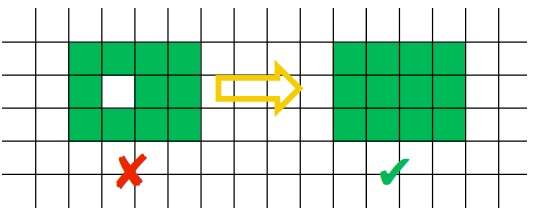

I don’t know how to deal with randomness in such a case. Perhaps one could try gaming the pseudorandom number generator, but it’s unlikely.

A perhaps more likely approach could be to start with a couple arbitrary guesses, compute probabilities for available cells find the next best guess that way, and try to evolve the grid to fit into desirable shape with a specific area. But such approach sounds complex, so instead I went for the (very) naive approach.

The RNG guesses uniformly, so probability that each of the 3x3 cells gets prepared is 1/9. So we could orient the 3x3 block in such a way that it always fits within the area we want to fully mark, and move the block from side to side, up and down, keeping guessing until we’re lucky and we fill the intended grid, or we run out of guesses. On the first visible test where N=20 it’s pretty likely that we’ll fill up a 4x5 grid, but I’m not so confident about the N=200 and 14x15 grid.

Something to keep in mind is how much of an overlap there is between two adjacent block guesses. The larger the overlap - the more likely overlapped cells will get marked, but the fewer guesses there are to cover the rest of the board. And edges and especially corners are a problem for such approach, as e.g. for a corner to be filled in there will only be as many opportunities as times one can cover the full board.

I first tried moving one column and one row at a time, and that was enough to pass the interactive local test and the visible test. But I was worried about corners and edges of the rectangle for the N=200 case, so instead I opted moving two columns and two rows at a time, reducing overlap between 2 adjacent guess blocks from 2 cells to 1 cell, but increasing the number of times the full board can be covered by about a factor of 2.

MAX_TRIES = 1000
HALT = 'HALT'

def has_test_failed(coords):
    return coords == [-1, -1]

def has_test_succeeded(coords):
    return coords == [0, 0]

def mark_filled_cell(cell, board):
    board[tuple(cell)] = True
    return board

def coords_offset(center, offset_x, offset_y):
    return (center[0]+offset_x, center[1]+offset_y)

def get_cell(coords, board):
    return tuple(coords) in board

def mask(center, board):
    """ List of cells in a guess block with a given center cell """
    result = []
    for i in range(3):
        for j in range(3):
            result.append(get_cell(coords_offset(center, i-1, j-1), board))
    return result

def solve(A):
    width = math.floor(math.sqrt(A))
    height = math.ceil(math.sqrt(A))
    WINDOW = 3
    board = {}
    guess = 0

    while guess < MAX_TRIES:
        # Leave out edges
        w = list(range(width))[1:-1]
        if width % 2 == 0: w.append(width - 1)
        h = list(range(height))[1:-1]
        if height % 2 == 0: h.append(height - 1)

        for i in w:
            for j in h:
                center = (i+1, j+1)
                if all(mask(center, board)):
                    # Given block is fully filled up
                    continue

                write_answer(center)
                filled_cell = read_ints()
                if has_test_failed(filled_cell):
                    return HALT
                if has_test_succeeded(filled_cell):
                    return
                board = mark_filled_cell(center, board)
                guess += 1
    return HALT

This passed 1 out of 2 tests, failing with a “Wrong answer” on the “N=200” hidden test. I didn’t expect the second one to pass - it was unlikely to do so. But, as a third option I would have tried placing guess blocks without any overlap at all, increasing the number of full rectangle guess coverage even further, in the hopes of hitting the right chance.

4. Cubic UFO

Problem description.

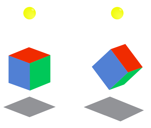
In short, there is a 3D cube hanging above ground and casting a shadow. How should we rotate the cube to get its shadow’s area to be as close as possible to a specific number? For simplicity’s sake, the cube’s center point is at origin (0, 0, 0), cube is 1km wide, and its shadow is being cast onto a screen 3km under the origin.

It was actually fairly straightforward, but tough to implement, requiring knowledge of multiple algorithms and implementation of matrix operations. I think I’ve spent most of my time on this problem.

The first idea was that maybe there is a mathematical formula describing an area of any cube slice through its center point. A quick search hasn’t yielded much, so this idea was abandoned.

Instead the requirements of the problem suggested a different approach. Notice that precision of answers has to be within about 10e-6, and inputs for all test cases are very precise, e.g. (1.000000, 1.414213, 1.732050). This raised an idea from numerical methods class - maybe if we could rotate the cube slightly, we could discover directions in which rotation gave the closest shadow area, and following those directions would get closer and closer to the desired answer.

From numerical methods class I vaguely remembered Newton’s method and from neural networks class came Gradient Descent.

On the right path, allowing to get closer and closer to the solution, but it’s only part of the solution. Full implementation still requires knowing how to calculate verteces and faces of the rotated cube, project those points onto 2D space, and calculate the area of cube’s shadow.

4.1. Cube rotations

First we need a way to describe the relevant coordinates. What would be the coordinates of each of the verteces and faces?

Well, cube’s center point is at origin, and the cube itself is 1km wide. That would mean its faces are 1km/2 = 0.5km away from the center point. So such points can be described as vectors, e.g. (0.5, 0, 0), (0, 0.5, 0), (0, 0, 0.5) vectors would give center points for three of the faces of the cube, and similarly replacing 0.5 with -0.5 would give the other 3 faces.

Likewise, cube’s verteces can be described as 3D vectors as well, e.g.: (0.5, 0.5, 0.5), (0.5, 0.5, -0.5), …, (-0.5, -0.5, -0.5).

So we have 2 sets of vectors, one to describe the 3 relevant face center points, and the other one for cube’s 8 verteces.

It’s been a while since my last linear algebra class, but after some searching I found that there are such things as Rotation matrices. Multiplying a vector by the appropriate rotation matrix would return the rotated vector. I would encourage you to read the full wiki article.

But doing so would require implementing some basic matrix functionality. Interestingly, as I was looking for solutions to this problem, many StackOverflow commentators suggested solutions using Numpy or Scikit, however such libraries are not available in Code Jam.

I’ve implemented matrices as follows. Matrix notation was [(a11, a21, ..., an1), (a12, ..., an2), ... (a1m, ..., anm)], where i denotes the row, and j denotes the column for a n row and m column (nxm) matrix. So the tuple in this case meant a column vector. Visually somewhat comfusing as they are written out in columns.

def matrix_column(A, column):
    return list(A[column])

def matrix_row(A, row):
    return list(map(lambda v: v[row], A))

def multiply_matrix(A, B):
    n = len(A[0])
    m = len(A)
    p = len(B)

    result = []
    for j in range(p):
        acc = []
        for i in range(n):
            c = 0
            for (a, b) in zip(matrix_row(A, i), matrix_column(B, j)):
                c += a * b
            acc.append(c)
        result.append(tuple(acc))

    return result

def test():
    # ...
    assert(multiply_matrix([(0, 0), (1, 0)], [(0, 1), (0, 0)]) == [(1, 0), (0, 0)])
    A = [(1, 4, 7), (2, 5, 8), (3, 6, 9)]
    assert(matrix_row(A, 2) == [7, 8, 9])
    assert(matrix_column(A, 2) == [3, 6, 9])
    assert(multiply_matrix([(1, 4, 7), (2, 5, 8), (3, 6, 9)], [(1, 2, 3)]) == [(14, 32, 50)])

Then following the Wikipedia article, matrix rotations can be described as:

def rotate_x(A, angle):
    R_x = [(1, 0, 0), (0, math.cos(angle), math.sin(angle)), (0, -1*math.sin(angle), math.cos(angle))]
    return multiply_matrix(R_x, A)

def rotate_y(A, angle):
    R_y = [(math.cos(angle), 0, -1*math.sin(angle)), (0, 1, 0), (math.sin(angle), 0, math.cos(angle))]
    return multiply_matrix(R_y, A)

def rotate_z(A, angle):
    R_z = [(math.cos(angle), math.sin(angle), 0), (-1*math.sin(angle), math.cos(angle), 0), (0, 0, 1)]
    return multiply_matrix(R_z, A)

def rotate_matrix(A, angle_x, angle_y, angle_z):
    return rotate_x(rotate_y(rotate_z(A, angle_z), angle_y), angle_x)

So now we can pass a matrix (e.g. cube’s verteces) into rotate_matrix along with 3 angles to rotate it in each of the 3 dimensions, and in the output we’d get the needed rotated vectors. The R_x, R_y and R_z rotation matrices were taken straight from the Wiki article, I haven’t looked too much into how they were derived - time was precious. But there we go, one step closer to the solution.

4.2. Area of the shadow

Now that in 4.1. we have calculated 3D coordinates of cube’s verteces, we can finally calculate the area of the shadow those coordinates define.

First we need to project 3D vertex points onto a 2D plane. The plane is on y=-3km, so conversion is as simple as omitting the y coordinate:

def project_3d_to_2d(vectors):
    # Skip y axis
    return list(map(lambda v: (round(v[0], 15), round(v[2], 15)), vectors))

round(x, 15) was used as a way to deal with floating point precision errors, where numbers should’ve been equal, but weren’t after a number of calculations. If you’re not familiar with floating point errors, you can read about them here. But, rounding the number to its 15th digit provided for enough precision.

Next, how to go from a set of points to calculating an area of the shape those points define? Sure, one may be able to calculate areas based on triangles between its points, or maybe integrate the area based on points.

I didn’t know this before, but it turns out that there’s such a thing as a Convex hull, which is an envelope of a set of points. And if you know that, you can calculate the area of the convex hull.

By Maonus CC BY-SA 4.0, from Wikimedia Commons

To find the convex hull of the shadow, I’ve followed the Gift-wrapping algorithm straight from the pseudocode provided in the Wiki article.

One more thing, to determine whether a point is on the left of the line, I’ve used this StackOverflow article. The resulting code looked like this:

def get_2d_convex_hull(S):
    def leftmost_point(S):
        return min(S, key=lambda p: p[0])

    def is_on_left(x, start, end):
        # is x on the left from line from start to end?
        return ((end[0] - start[0])*(x[1] - start[1]) - (end[1] - start[1])*(x[0] - start[0])) > 0

    P = []
    point_on_hull = leftmost_point(S)
    i = 0
    while True:
        P.append(point_on_hull)
        endpoint = S[0]
        for j in range(len(S)):
            if endpoint == point_on_hull or is_on_left(S[j], P[i], endpoint):
                endpoint = S[j]
        i += 1
        point_on_hull = endpoint

        if endpoint == P[0]:
            break

    return P

And to find the area of the convex hull, another StackOverflow article came to the rescue:

def get_convex_hull_area(S):
    def area(p):
        return 0.5 * abs(sum(x0*y1 - x1*y0
                             for ((x0, y0), (x1, y1)) in segments(p)))

    def segments(p):
        return zip(p, p[1:] + [p[0]])

    return area(S)

Great! Now we can rotate the cube to a specific angle, and calculate what is the area of its shadow.

4.3. Cube shadow’s area

Putting 4.1. and 4.2. together we can calculate the area of cube’s shadow once it’s rotated to a specific angle:

def get_step(angle_alpha, angle_beta, angle_gamma):
    faces = [(0.5, 0, 0), (0, 0.5, 0), (0, 0, 0.5)]
    verteces = [
        (0.5, 0.5, 0.5), (0.5, 0.5, -0.5),
        (0.5, -0.5, 0.5), (0.5, -0.5, -0.5),
        (-0.5, 0.5, 0.5), (-0.5, 0.5, -0.5),
        (-0.5, -0.5, 0.5), (-0.5, -0.5, -0.5)
    ]

    new_faces = rotate_matrix(faces, angle_alpha, angle_beta, angle_gamma)
    new_verteces = rotate_matrix(verteces, angle_alpha, angle_beta, angle_gamma)

    projected_verteces = project_3d_to_2d(new_verteces)

    hull = get_2d_convex_hull(list(set(projected_verteces)))
    area = get_convex_hull_area(hull)

    return {
        'faces': new_faces,
        'area': area,
    }

We start with the initial cube, and then rotate both face and vertex vectors to the same angle. We’ll use vertex vectors for optimization, while face vectors will be necessary for the answer.

3D vertex vectors are converted to 2D ones by omitting the Y coordinate, and then that matrix is turned into a set to eliminate duplicate coordinates.

The function is named get_step(), as we will iteratively change all three angles by small amounts to find the right values such that the area is as close to the desired target as we can get.

4.4. Function optimization

The goal is to find angles alpha, beta and gamma, so that get_step(alpha, beta, gamma) gives an answer close to the target value. So the smaller abs(target - get_step(alpha, beta, gamma) is - the better our answer is.

There are a number of algorithms to consider. I looked into Gradient descent I knew a bit about from Neural Network classes, but that didn’t work.

After some searching I found an implementation for Continuous hill climbing and Random Optimization. I went for a slightly modified version of Continuous hill climbing algorithm.

Upon implementation of the exact same hill climbing algorithm from the wiki article I found that it tended to always converge to 1.732050, which seems to be the maximum area the shadow can cover, even though the target was different. So I had to modify scoring slightly.

The original hill climbing algorithm starts from -infinity and tries to climb up. Because our goal is to get to zero, I changed the algorithm to start from +infinity, and modified best_score evaluation to: evaluate = lambda score: abs(score - target)

The idea of the algorithm is fairly simple. In each iteration it tries to nudge a single variable in some direction. If doing so gives a better scoring answer than it had before - then it uses that newly discovered point for the next iteration, gradually inching closer and closer to the goal.

It can be implemented as follows:

def solve(target):
    df = lambda alpha, beta, gamma: get_step(alpha, beta, gamma)['area']
    evaluate = lambda score: abs(score - target)
    alpha = 0
    beta = 0
    gamma = 0

    PRECISION = 10e-10
    current_point = [1, 1, 1]
    step_size = [1, 1, 1]
    acceleration = 12
    candidate = [-acceleration, -1 / acceleration, 0, 1 / acceleration, acceleration]

    while True:
        before = df(*current_point)
        for i in range(len(current_point)):
            best = -1
            best_score = math.inf

            for j in range(5):
                current_point[i] += step_size[i] * candidate[j]
                temp = df(*current_point)
                current_point[i] -= step_size[i] * candidate[j]
                if evaluate(temp) < best_score:
                    best_score = evaluate(temp)
                    best = j

            if candidate[best] == 0:
                step_size[i] /= acceleration
            else:
                current_point[i] += step_size[i] * candidate[best]
                step_size[i] *= candidate[best]

        t = df(*current_point)
        if abs(target - t) < PRECISION:
            solution = get_step(*current_point)
            return solution['faces']

    return []

And turns out, in this case it converges fairly quickly to the target 1.414213:

Area               Error
1.4091240054698353 0.005088994530164648
1.4119704586438513 0.002242541356148653
1.4126303658805988 0.0015826341194011828
1.414195691609093 1.730839090696712e-05
1.4142002234618065 1.277653819342639e-05
1.4142116144140569 1.385585943092238e-06
1.414212563509047 4.3649095293751827e-07
1.4142130175986523 1.7598652313211005e-08
1.4142129999828152 1.7184698108962948e-11

Answer:
[(0.16611577741917438, 0.47116771198777596, -0.020162729791066175), (-0.2584057051447727, 0.1088197672910437, 0.4139864125733548), (0.394502268740062, -0.12711902071258785, 0.27965821019955156)]

Or to 1.732050:

Area              Error
1.721904229213536 0.010145770786464059
1.723231518102203 0.008818481897796993
1.731250867053177 0.0007991329468231001
1.731673628707239 0.0003763712927611351
1.7316954153046518 0.0003545846953483256
1.7318965769362784 0.00015342306372168046
1.7319103991653426 0.00013960083465747175
1.7320214355685835 2.856443141663334e-05
1.7320272993244448 2.2700675555320515e-05
1.7320482657017473 1.7342982527868145e-06
1.7320496821790208 3.1782097931198905e-07
1.7320497962679902 2.037320099290696e-07
1.732049804975619 1.9502438108887077e-07
1.7320498998698852 1.0013011486620371e-07
1.7320499073756168 9.262438327439781e-08
1.7320499949575732 5.0424269204540906e-09
1.732050001429884 1.4298839889903547e-09
1.7320500000601848 6.018474607571989e-11

Answer:
[(0.17916829614835567, 0.28883339349608833, 0.3667069571971998), (-0.22756542797063706, -0.28890843314528813, 0.3387416320000767), (0.40756925503260905, -0.2882831733887158, 0.02793052618723268)]

This solution worked for both tests, succeeding in 2/2 tests and getting 32 points. Only 1158 contestants solved both correctly, I’m happy to be one of them.

Final thoughts

Overall, it was fun. Not too happy about my performance with the first two problems, I think I could’ve gotten them if I was more attentive.

The last problem, just like in the Practice round, was tough, but satisfying to solve, and I’ve certainly learned a lot.

First is the value of knowing how such algorithms work and being able to implement them yourself. Sure, having a library take care of it is convenient, but one still needs to know what’s under the hood. Matrix operations, finding the convex hull and its area, function optimization were the big ones.

In the end I’ve solved all 4 problems, but got both test cases only for the last one (first: 1/2, second: 1/2, third: 1/2, fourth: 2/2). I got a total score of 55/100 and placed 5872/21300. Over 24 thousand people have participated in this round, which is way more than 4199 in the Practice round. Unexpected!

Considering that it took me about 10 hours for all 4 problems and that the first round’s duration is only 2 hours, I’m not sure I’ll participate in the next round. But, anyone who got more than 25 points will be invited to the next round, so we’ll see.

All in all I think it was a decent investment of a half of a weekend. And if you would like to crack your brain on some programming problems too, consider joining Google Code Jam next year, the event is organized yearly.

And if you have participated in the competition, how did you approach these problems?

If you’re not familiar with Google Code Jam, it’s a yearly competition organized by Google where contestants compete in solving programming problems. You are given a problem and some limitations, e.g. only a few hours to prepare solutions in later stages of the event, runtime and memory constraints for programs. It’s a fairly popular contest, bringing in thousands of participants from all over the world, with World Finals taking place in Toronto and the best contestant taking home a $15,000 grand prize, fame and glory.

In the practice session of 2018 there were 4 problems and 2 days were given to solve them. You can find the full list of problems and their descriptions HERE.

1. Number Guessing

Here’s the full problem description.

But in short, the judge program comes up with a secret number in a given range and allows you to make no more than a specific number of guesses. Your program has to guess what the number is, and after each guess the judge will respond with “TOO_BIG”, “TOO_SMALL” or “CORRECT”. If your program fails to guess the number correctly, the judge will respond with “WRONG_ANSWER” and will stop replying.

This immediately sounds like binary search, doesn’t it? You have to guess a number in 1-dimensional space, and the only feedback judge provies is if we guessed to high or too low. So the best we can do is to always guess in the middle of the available space, discarding the half where we know our target is not in. Based on the image example above, it would take 4 guesses to find the right answer using this strategy: binary search has an average performance of O(log(n)).

My first stumble was in picking the right midpoint. Initial one was the average of lower and upper bounds midpoint = (lower_bound + upper_bound) // 2. Integer division is there to avoid producing a decimal number (e.g. (1 + 4) / 2 == 2.5, but (1 + 4) // 2 == 2). This passed the testing_tool.py, but failed hidden tests, failing to find the answer in required number of guesses. Wiki article also suggests using floor of (lower_bound + upper_bound) / 2, but taking ceil instead passed the tests: midpoint = (lower_bound + upper_bound + 1) // 2.

The second stumble was in not terminating the program as specified when the judge responded with WRONG_ANSWER. It wasn’t quite clear whether on the last answer it would respond with TOO_BIG and then WRONG_ANSWER, or just WRONG_ANSWER, so I covered for both, yielding this code:

def run():
    test_cases = read_int()
    for case in range(test_cases):
        case += 1
        [lower_bound, upper_bound] = read_ints()
        guesses = read_int()

        guessed_right = False

        for guess in range(guesses):
            midpoint = (lower_bound + upper_bound + 1) // 2
            write_guess(midpoint)

            answer = read_answer()

            if answer == TOO_BIG:
                upper_bound = middle
            elif answer == TOO_SMALL:
                lower_bound = middle
            elif answer == CORRECT:
                guessed_right = True
                break
            elif answer == WRONG_ANSWER:
                exit()

        if guessed_right == False:
            answer = read_answer()
            exit()

I skipped definitions for read_int(), read_ints(), read_answer(), write_guess() - they’re basic stdin and stdout operations.

2. Senate evacuation

Here’s the full problem description.

In short, there are a number of political parties in senate with some number of senators in each party. We want to evacuate all senators in such a way that neither party has the majority at any step (>50% of senators still in senate), while we can evacuate only one or two senators at a time.

Or to rephrase the problem slightly differently: we have a list of integers, we can subtract 1 or 2 at a time from any member in such a way that neither member is bigger than 50% of sum of all members. Let’s start with checking the current state for validity and encode this rephrased version in code:

def is_valid(senators):
    total_senators = sum(senators)
    limit = total_senators / 2
    return all(map(lambda p: p <= limit, senators))

For the strategy itself, initial hunch suggests to attack parties with most senators first. We will always be able to evacuate at least one senator. As for the second one, after selecting the first candidate we can check again which party has most members. If after removing it the state is still legal (using is_valid()) - then we can take two senators. If not - we have to take just one. We just have to take into account a case when there are no senators left at all ([0, 0, ..., 0]), or just one ([1, 0, 0, ..., 0]). In code this idea can be written as:

def solve(parties, senators):
    solution = []
    most_senators = max(senators)
    while most_senators > 0:
        first_target = senators.index(most_senators)
        senators[first_target] -= 1

        second_largest_party = max(senators)
        second_target = senators.index(second_largest_party)
        senators[second_target] -= 1

        if second_largest_party == 0 or not is_valid(senators):
            # Can take only one senator, must put second one back
            solution.append(alphabet[first_target])
            senators[second_target] += 1
        else:
            # Can take both senators
            solution.append(alphabet[first_target] + alphabet[second_target])

        most_senators = max(senators)
    return solution

And to transform political party numbers back into alphabetical party names: alphabet = dict(enumerate('ABCDEFGHIJKLMNOPQRSTUVWXYZ')).

With final run() written as:

def run():
    test_cases = read_int()
    for case in range(test_cases):
        case += 1
        N = read_int()
        senators = read_ints()
        solution = solve(N, senators)

        write_answer('Case #%d: %s' % (case, ' '.join(solution)))

3. Steed 2: Cruise Control

Here’s the full problem description.

In short, on a one-way road there are a number of horses with some initial positions and all travelling in the same direction at some individual speeds. However, these horses move in a special way in that they cannot pass each other. So if one catches up to another, they’ll both continue travelling at the slower one’s speed. Our hero wants to travel to a specific point on the same road and has to abide same rules of not passing another horse. The hero can travel at any speed, but wants to maintain a constant speed throughout the full travel without having to speed up or slow down. What is the maximum speed the hero can choose?

The first hunch was to try and calculate for how long each horse will travel at what speed, and try to deduce hero’s target speed from that. But the problem mentions that it may use up to 1000 horses. At least we can imagine describing a situation where we put fastest horses at the start, and slowest ones near the end, and faster horses gradually running into slower ones. It quickly becomes a complex mess.

The second idea was to compute how long it will take for each horse to get to hero’s destination, but do it from right to left. Right to left, because horses to the right will always be limiting factors - horses to the left can’t get to the destination faster than the horse to the right, they’d eventually catch up and will have to slow down, so their journey will take at least as long as the horse’s to the right. And turns out that this approach allows for fairly straightforward linear computation.

So for each horse we compute how long it would take them to cover the remaining distance from their starting point to the destination. If we take the max() of these durations, that will give us our hero’s travel duration. From there we can find the average speed with average_speed = distance / duration.

def solve(distance, total_horses, horses):
    longest_duration = max(map(lambda h: (distance - h[0]) / h[1], horses.values()))
    return distance / longest_duration

def run():
    test_cases = read_int()
    for case in range(test_cases):
        case += 1
        [distance, total_horses] = read_ints()
        horses = {}
        for i in range(total_horses):
            [initial, max_speed] = read_ints()
            horses[i] = [initial, max_speed]
        # print([distance, total_horses, horses])
        solution = solve(distance, total_horses, horses)

        write_answer('Case #%d: %.7f' % (case, solution))

4. Bathroom Stalls

Here’s the full problem description.

In short, there are N+2 bathroom stalls, with first and last one already occupied. A number of people will come in one after another, selecting a stall and never leaving. People will select a stall that is furthest from its closest neighbors. The goal is to find out, when the last person takes a stall, what’s the largest and lowest number of free stalls next to the side of it.

This one was rough, taking about 4 hours to figure out, but in the end the solution was mathematical and fairly elegant, at least in my eyes.

The initial idea would be to maybe try and write a program that puts people in the appropriate stalls sequentially one by one. But the problem arises from constraints: the number of stalls can be as large as 10^18, and number of people can be equal to the number of stalls.

How would such data structure be represented? If we represented each stall as 1 byte, that’s still 10^18 bytes - exabyte, for comparison a gigabyte is about 10^9, so there’s no way we’re storing this much information, in memory or on disk. northeastern.edu suggests that in 2013 total amount of data in the world was 4.4 zettabytes, or 4400 exabytes. We certainly won’t dedicate 0.2% of world’s storage to solve this problem. And If each stall was represented as a bit, divide the numbers by 8, but they’re still gargantuan and unmanageable numbers.

Especially note that the execution time limit is 30 seconds. Which suggests there has to be a better way.

The next idea was that maybe it could be related to fractals - similar repeating patterns at different scales. E.g. Here’s how 7 stalls would be filled up:

1|2|3|4|5|6|7  1|2|3|4|5|6|7
-------------  -------------
_|_|_|1|_|_|_  _|_|_|1|_|_|_
_|2|_|_|_|_|_  _|2|_|1|_|_|_
_|_|_|_|_|3|_  _|2|_|1|_|3|_
4|_|_|_|_|_|_  4|2|_|1|_|3|_
_|_|5|_|_|_|_  4|2|5|1|_|3|_
_|_|_|_|6|_|_  4|2|5|1|6|3|_
_|_|_|_|_|_|7  4|2|5|1|6|3|7

Maybe the same pattern that governs selection of one could be repeated on its left branch to position 2, resulting maybe in a tree of sorts. But that still does not suggest a way how to determine number of free stalls on each position’s side. So the third option was to brute force and write down free stall numbers for each N.

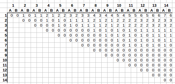
In the graph the columns denote N - how many stalls there are. Rows denote how many people have already selected a stall. And (stalls, people) combination denotes A - the largest number of stalls available next to last person’s stall, and B - the lowest number of stalls next to the last selected stall.

Right away we see an interesting trend. E.g. take a look at the first row. As columns grow from left to right, first A increases by one, then B catches up on the next column. And it repeats.

On the second row it’s very similar. First A increases by one, then B catches up, but this rate of change is slower, only every two columns as opposed to with every one.

It’s getting difficult to follow, as we’re running out of columns to clearly see the trend, but on the fourth row the rate of change is even slower, with A and B incrementing only once every 4 columns.

Let’s add some visual aid:

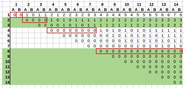
It would be a bit clearer if we had 16 rows and 16 columns, but this suffices to spot the trend.

We can see that rate of change also changes based on the row, and such rates of change can be grouped based on powers of two:

• 2^0 = 1 - one row will change on every column;
• 2^1 = 2 - there are 2 rows in the group, so A and B wil change every 2 columns on rows 2 and 3;
• 2^2 = 2 - there are 4 rows in the group, A and B will change every 4 columns on rows 4-7;
• 2^3 = 8 - there are 8 rows in the group, A and B will change every 8 columns on rows 8-15;

And so on. We have found a pattern. Now how to calculate A and B if we are given the row and column number?

Rate of change

First we need to find every how many columns A and B changes based on the row. Since groups grow as powers of two, we could take floor(log2(row)) to find in which group a row is. E.g. floor(log2(9)) = 3, which means we are in the fourth group (indexed from 0, see list above). If we raise the base 2 back to the power of 3 - this gives us rate of change 8, which is what we would expect as per our pattern we’ve seen above.

So the derived formula for rate of change seems to be rate_of_change = lambda row: 2 ** math.floor(math.log2(row))

How many changes already occurred

Next we need to find out how many changes have occurred based on the column number. We can see that A and B always change in the following pattern:

0 0 -> 1 0 -> 1 1 -> 2 1 -> 2 2 -> 3 2 -> 3 3 -> ... -> x+1 x -> x+1 x+1 -> ...

So based on rate of change we can count how many changes have already occurred given a row and a column.

Taking a look at the stall positioning table again, for any row number, on which column does the row start? We see that the row starts at the column number equal to the row number. E.g. row 4 starts at 4th column, row 9 starts at 9th column. So if we check how many rate_of_change columns fit in this space - that will tell us how many changes have already occurred.

E.g. for row=3, column=6, the rate of change is 2 ** math.floor(math.log2(3)) == 2. Row 3 starts at column 3, and we’re interested in column 6. 6-3 leaves a space of 3 for changes to occur in. If we divide that by rate_of_change = 2 => (6 - 3) / 2 = 1.5. So a full one change has already occurred, going 0 0 -> 1 0. If you check the table again, we see that this is exactly right.

So the derived formula seems to be number_of_changes_done = lambda column, row: math.floor((column - row) / rate_of_change(row))

Putting it all together: calculating A and B

Now we can calculate A and B.

If we take a look at the first line, we see that A number seems to be equal to about half of the number of changes for a specific column. E.g. on row=1 column=3, the result we are aiming for is A=1, B=1, and a total of 2 changes have already occurred. Or on row=1 column=10, the result we are aiming for is A=5, B=4, and a total of 9 changes have already occurred.

And B tends to also be about half of the number of changes for a specific column, but always either equal to A, or one less than A.

So my idea was to use ceil and floor, setting A = math.ceil(number_of_changes_done / 2), and B = number_of_changes_done - A, and this seems to work.

E.g. row=1 column=3: number_of_changes_done = 2, A = math.ceil(2 / 2) => math.ceil(1) => 1, B = 2 - 1 => B = 1. Or row=6, column=14: number_of_changes_done = 2, A = math.ceil(2 / 2) => math.ceil(1) => 1, B = 2 - 1 => B = 1. Or row=2, column=11: number_of_changes_done = 4, A = math.ceil(4 / 2) => math.ceil(2) => 2, B = 4 - 2 => B = 2.

The formulas seem to check out!

Final code

def get_change_rate_on_row(K):
    # Every how many records do values change on row K
    return 2 ** math.floor(math.log2(K))

def number_of_changes_done(N, K):
    return math.floor((N - K) / get_change_rate_on_row(K))

def solve(N, K):
    change_rate = get_change_rate_on_row(K)

    total_changes = number_of_changes_done(N, K)

    y = math.ceil(total_changes / 2)
    z = total_changes - y

    return [str(y), str(z)]

def run():
    test_cases = read_int()
    for case in range(test_cases):
        case += 1
        [stalls, people] = read_ints()

        solution = solve(stalls, people)

        # print(case, solution)
        write_answer('Case #%d: %s' % (case, ' '.join(solution)))

All this work for a straight forward calculation! But there we go, we have calculated values A and B for any given row and column in a fraction of a second and without using 0.02% of world’s data storage capacity.

Final thoughts

The final result ended up being:

• Place: 661/4199
• Score: 60
• Problem 1: 2/2
• Problem 2: 2/2
• Problem 3: 2/2
• Problem 4: 2/3. Last test with 1 <= N <= 10^18 failed with “Wrong answer”. Unfortunately data is not published, so I can’t check what happened, especially at that scale.

But overall it’s been a fun brain teaser. The last problem was especially challenging, but that made it so much more satisfying to crack.

The first problem seemed like a clear approach for binary search, but I was unable to think of any metaphors or similar problems for the other three. I managed to muddle through them, but seeing how quickly other contestands were able to breeze through these problems, that makes me think that there are other relatable problems or approaches one could use here. Have you solved these problems? What approach did you take? I’d be curious to learn more.

And if you haven’t tried Google Code Jam or similar competitions before - give it a go some time. They can twist your brain unlike daily CRUD apps, making us more capable of solving more complex problems in the end.

In multiplayer games bots have been popular in giving an edge to players on certain tasks, like farming in-game currency in World of Warcraft, Eve Online, level up bots for Runescape. As a technical challenge it can be as basic as a program to play Tic Tac Toe for you, or as complex as DeepMind and Blizzard using StarCraft II as their AI research environment.

If you are interested in getting your feet wet with Computer Vision, game automation can be an interesting and fairly easy way to practice: contents are predictable, well known, new data can be easily generated, interactions with the environment can be computer controlled, experiments can be cheaply and quickly tested. Grabbing new data can be as easy as taking a screenshot, while mouse and keyboard can be controlled with multiple languages.

In this case we will use the most basic strategy in CV - template matching. Of course, depends on the problem domain, but the technique can be surprisingly powerful. All it does is it slides the template image across the input image and compares differences. See Template matching docs for more visual explanation of how it works.

As the test bed I’ve chosen a flash game called Burrito Bison. If you’re not familiar with it - check it out. The goal of the game is to throw yourself as far as possible, squishing gummy bears along the way, earning gold, buying upgrades and doing it all over again. Gameplay itself is split into multiple differently themed sections, separated by giant doors, which the player has to gain enough momentum to break through.

It is a fairly straightforward game with basic controls and a few menu items. Drag the bison for it to jump off the ropes and start the game, left-click (anywhere) when possible to force smash gummy bears, buy upgrades to progress. No keyboard necessary, everything’s in 2D, happening on a single screen without the need for player to manually scroll. The somewhat annoying part is having to grind enough gold coins to buy the upgrades - it is tedious. Luckily it involves few actions and can be automated. Even if done suboptimally - quantity over quality, and the computer will take care of the tediousness.

If you are interested in the code, you can find the full project on Github.

Overview and approach

Let’s first take a look at what needs to be automated. Some parts may be ignored if they don’t occur frequently, e.g. starting the game itself, some of the screens (e.g. item unlocked). But can be handled if desired.

There are 3 stages of the game with multiple screens, multiple objects to click on. Thus the bot will sometimes need to look for certain indicators whether or not it’s looking at the right screen, or look for objects if it needs to interact with them. Because we are working with templates, any changes in dimensions, rotation or animations will make it more difficult to match the objects. Thus objects bot looks for have to be static.

1. Starting the round

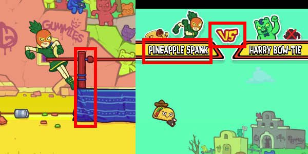
The round is started by pushing the mouse button down on the bison character, dragging the character to aim and releasing it. If bison hit the “opponent” - a speed boost is provided.

There are several objects to think about:

1. Bison itself. The bot will need to locate the bison character and drag it away to release it
2. Whether or not the current screen is the round starting screen. Because the player character will occur elsewhere in the game, the bot may be confused and misbehave if we use the bison itself. A decent option could be to use ring’s corner posts or the “vs” symbol.

2. Round in progress

Once the round has started, the game plays mostly by itself, no need for bot interactions for the character to bounce around.

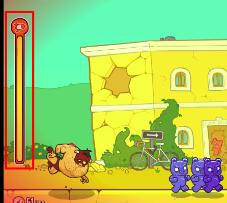
To help gain more points though we can use the “Rocket” to smash more gummies. To determine when rocket boost is ready we can use the full rocket boost bar as a template. Left mouse click anywhere on screen will trigger it.

3. Round ended

Once the round ends there are be a few menu screens to dismiss (pinata ad screen, missions screen, final results screen), and the bot will need to click a button to restart the round.

Pinata screen:

• we can use “I’m filled with goodies” text as the template to determine if we’re on the pinata screen. Pinata animation itself moves, glows, which may make it difficult for bot to match to template, thus unsuitable.
• “Cancel” button, so the bot can click it

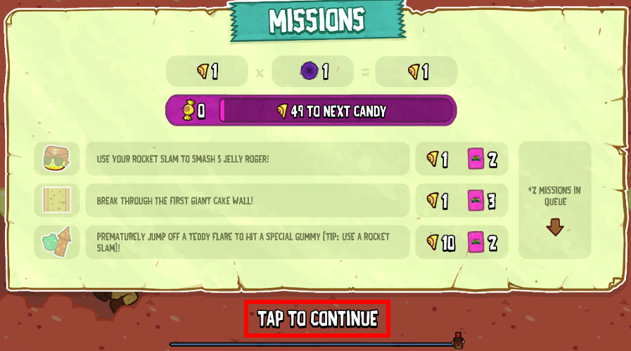
Mission screen:

Simply match the “Tap to continue” to determine if we’re on this particular screen and left mouse click on it to continue.

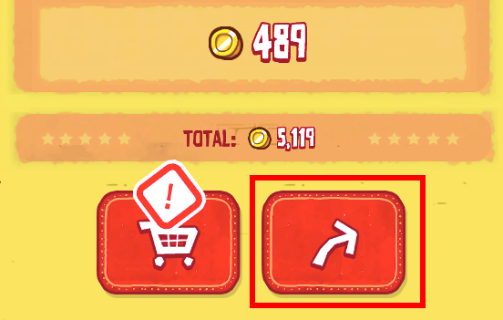
Round results screen:

Here “Next” button is static and we can reliably expect it to be here based on game’s flow. The bot can match and click it.

Implementation

For vision we can use OpenCV, which has Python support and is the defacto library for computer vision. There’s plenty to choose from for controlling the mouse, but I found luck with Pynput.

Controls

As far as controls go, there are 2 basic actions bot needs to perform with the mouse: 1) Left click on a specific coordinate 3) Left click drag from point A to point B

Let’s start with moving the mouse. First we create the base class:

import time
from pynput.mouse import Button, Controller as MouseController

class Controller:
    def __init__(self):
        self.mouse = MouseController()

The Pynput library allows setting mouse position via mouse.position = (5, 6), which we can use. I found that in some games changing mouse position in such jumpy way may cause issues with events not triggering correctly, so instead I opted to linearly and smoothly move the mouse from point A to point B over a certain period:

    def move_mouse(self, x, y):
        def set_mouse_position(x, y):
            self.mouse.position = (int(x), int(y))
        def smooth_move_mouse(from_x, from_y, to_x, to_y, speed=0.2):
            steps = 40
            sleep_per_step = speed // steps
            x_delta = (to_x - from_x) / steps
            y_delta = (to_y - from_y) / steps
            for step in range(steps):
                new_x = x_delta * (step + 1) + from_x
                new_y = y_delta * (step + 1) + from_y
                set_mouse_position(new_x, new_y)
                time.sleep(sleep_per_step)
        return smooth_move_mouse(
            self.mouse.position[0],
            self.mouse.position[1],
            x,
            y
        )

The number of steps used here is likely too high, considering the game should be capped at 60fps (or 16.6ms per frame). 40 steps in 200ms means a mouse position change every 5ms, perhaps redundant, but seems to work okay in this case.

Left mouse click and dragging from point A to B can be implemented using it as follows:

    def left_mouse_click(self):
        self.mouse.click(Button.left)

    def left_mouse_drag(self, start, end):
        self.move_mouse(*start)
        time.sleep(0.2)
        self.mouse.press(Button.left)
        time.sleep(0.2)
        self.move_mouse(*end)
        time.sleep(0.2)
        self.mouse.release(Button.left)
        time.sleep(0.2)

Sleeps in between mouse events help the game keep up with the changes. Depending on the framerate these sleep periods may be too long, but compared to humans they’re okay.

Vision

I found the vision part to be the most finicky and time consuming. It helps to save problematic screenshots and write tests against them to ensure objects get detected as expected. During bot’s runtime we’ll use MSS library to take screenshots and perform object detection on them with OpenCV.

import cv2
from mss import mss
from PIL import Image
import numpy as np
import time

class Vision:
    def __init__(self):
        self.static_templates = {
            'left-goalpost': 'assets/left-goalpost.png',
            'bison-head': 'assets/bison-head.png',
            'pineapple-head': 'assets/pineapple-head.png',
            'bison-health-bar': 'assets/bison-health-bar.png',
            'pineapple-health-bar': 'assets/pineapple-health-bar.png',
            'cancel-button': 'assets/cancel-button.png',
            'filled-with-goodies': 'assets/filled-with-goodies.png',
            'next-button': 'assets/next-button.png',
            'tap-to-continue': 'assets/tap-to-continue.png',
            'unlocked': 'assets/unlocked.png',
            'full-rocket': 'assets/full-rocket.png'
        }

        self.templates = { k: cv2.imread(v, 0) for (k, v) in self.static_templates.items() }

        self.monitor = {'top': 0, 'left': 0, 'width': 1920, 'height': 1080}
        self.screen = mss()

        self.frame = None

First we start with the class. I cut out all of the template images for objects the bot will need to identify and stored them as png images.

Images are read with cv2.imread(path, 0) method, where the zero argument will read those images as grayscale, which simplifies the search for OpenCV. As a matter of fact, the bot will only work with grayscale images. And since these template images will be used frequently, we can cache them on initialization.

Configuration for MSS is hardcoded here, but can be changed or extracted into a constructor argument if we want to.

Next we add a method to take screenshots with MSS and convert them into grayscale images in the form of Numpy arrays:

    def convert_rgb_to_bgr(self, img):
        return img[:, :, ::-1]

    def take_screenshot(self):
        sct_img = self.screen.grab(self.monitor)
        img = Image.frombytes('RGB', sct_img.size, sct_img.rgb)
        img = np.array(img)
        img = self.convert_rgb_to_bgr(img)
        img_gray = cv2.cvtColor(img, cv2.COLOR_BGR2GRAY)

        return img_gray

    def refresh_frame(self):
        self.frame = self.take_screenshot()

RGB to BGR color conversion is necessary, as while the MSS library will take screenshots using RGB colors, OpenCV uses BGR colors. Skipping the conversion will usually result in incorrect colors. And refresh_frame() will be used by our game class to instruct when to fetch a new screenshot. This is to avoid taking and processing screenshots with every template matching call, as it is an expensive operation after all.

To match templates within screenshots we can use the built-in cv2.matchTemplate(image, template, method) method. It may return more matches that may not fully match, but those can be filtered out.

    def match_template(self, img_grayscale, template, threshold=0.9):
        """
        Matches template image in a target grayscaled image
        """

        res = cv2.matchTemplate(img_grayscale, template, cv2.TM_CCOEFF_NORMED)
        matches = np.where(res >= threshold)
        return matches

You can find more about how different matching methods work on OpenCV documentation

To simplify work with matching our problem domain’s templates we add a helper method which will use a template picture when given its name:

    def find_template(self, name, image=None, threshold=0.9):
        if image is None:
            if self.frame is None:
                self.refresh_frame()

            image = self.frame

        return self.match_template(
            image,
            self.templates[name],
            threshold
        )

And while the reason is not obvious yet, let’s add a different variation of this method which would try to match at least one of rescaled template images. As we’ll later see, at the start of the round camera’s perspective may change depending on size of the opponent, making some objects slightly smaller or larger than our template. Such bruteforce method of checking templates at different scales is expensive, but in this use case it seemed to work acceptably while allowing to continue using the simple technique of template matching.

    def scaled_find_template(self, name, image=None, threshold=0.9, scales=[1.0, 0.9, 1.1]):
        if image is None:
            if self.frame is None:
                self.refresh_frame()

            image = self.frame

        initial_template = self.templates[name]
        for scale in scales:
            scaled_template = cv2.resize(initial_template, (0,0), fx=scale, fy=scale)
            matches = self.match_template(
                image,
                scaled_template,
                threshold
            )
            if np.shape(matches)[1] >= 1:
                return matches
        return matches

Game logic

There are several distinct states of the game:

• not started/starting
• started/in progress
• finished (result screens)

Since game linearly follows these states every time, we can use them to limit our Vision to check only for objects the bot can expect to find based on state it thinks the game is in. It starts with not started state:

import numpy as np
import time

class Game:

    def __init__(self, vision, controller):
        self.vision = vision
        self.controller = controller
        self.state = 'not started'

Next we add a few helper methods to check if object exists based on template, and to attempt to click on that object:

    def can_see_object(self, template, threshold=0.9):
        matches = self.vision.find_template(template, threshold=threshold)
        return np.shape(matches)[1] >= 1

    def click_object(self, template, offset=(0, 0)):
        matches = self.vision.find_template(template)

        x = matches[1][0] + offset[0]
        y = matches[0][0] + offset[1]

        self.controller.move_mouse(x, y)
        self.controller.left_mouse_click()

        time.sleep(0.5)

Nothing fancy, the heavy lifting is done by OpenCV and Vision class. For object clicking offsets, they usually will be necessary as (x, y) coordinates will be for the top left corner of the matched template, which may not always be in the zone of object activation in-game. Of course, one could center the mouse on template’s center, but object-specific offsets work okay as well.

Next let’s run over indicator objects, and objects the bot will need to click on:

• Character’s name on the health bar (indicator whether the round is starting);
• Left corner post of the ring (to launch the player). Tried using character’s head before, but there are multiple characters in rotation as game progresses;
• “Filled with goodies!” text (indicator for pinata screen);
• “Cancel” button (to exit pinata screen);
• “Tap to continue” text (to skip “Missions” screen);
• “Next” button (to restart round);
• Rocket bar (indicator for when rocket boost can be launched);

These actions and indicators can be implemented with these methods:

    def round_starting(self, player):
        return self.can_see_object('%s-health-bar' % player)

    def round_finished(self):
        return self.can_see_object('tap-to-continue')

    def click_to_continue(self):
        return self.click_object('tap-to-continue', offset=(50, 30))

    def can_start_round(self):
        return self.can_see_object('next-button')

    def start_round(self):
        return self.click_object('next-button', offset=(100, 30))

    def has_full_rocket(self):
        return self.can_see_object('full-rocket')

    def use_full_rocket(self):
        return self.click_object('full-rocket')

    def found_pinata(self):
        return self.can_see_object('filled-with-goodies')

    def click_cancel(self):
        return self.click_object('cancel-button')

Launching the character is more involved, as it requires dragging the character sideways and releasing. In this case I’ve used the left corner post instead of the character itself because there are two characters in rotation (Bison and Pineapple).

    def launch_player(self):
        # Try multiple sizes of goalpost due to perspective changes for
        # different opponents
        scales = [1.2, 1.1, 1.05, 1.04, 1.03, 1.02, 1.01, 1.0, 0.99, 0.98, 0.97, 0.96, 0.95]
        matches = self.vision.scaled_find_template('left-goalpost', threshold=0.75, scales=scales)
        x = matches[1][0]
        y = matches[0][0]

        self.controller.left_mouse_drag(
            (x, y),
            (x-200, y+10)
        )

        time.sleep(0.5)

This is where the bruteforce attempt comes in to detect different scales of templates. Previously I used the same template detection using self.vision.find_template(), but that seemingly randomly failed. What I ended up noticing is that depending on the size of the opponent affects camera’s perspective, e.g. first green bear is small and static, while brown bunny jumps up significantly. So for bigger opponents camera zoomed out, making the character smaller than the template, while on smaller opponents the character became larger. So such broad range of scales is used in an attempt to cover all character and opponent combinations.

Lastly, game logic can be written as follows:

    def run(self):
        while True:
            self.vision.refresh_frame()
            if self.state == 'not started' and self.round_starting('bison'):
                self.log('Round needs to be started, launching bison')
                self.launch_player()
                self.state = 'started'
            if self.state == 'not started' and self.round_starting('pineapple'):
                self.log('Round needs to be started, launching pineapple')
                self.launch_player()
                self.state = 'started'
            elif self.state == 'started' and self.found_pinata():
                self.log('Found a pinata, attempting to skip')
                self.click_cancel()
            elif self.state == 'started' and self.round_finished():
                self.log('Round finished, clicking to continue')
                self.click_to_continue()
                self.state = 'mission_finished'
            elif self.state == 'started' and self.has_full_rocket():
                self.log('Round in progress, has full rocket, attempting to use it')
                self.use_full_rocket()
            elif self.state == 'mission_finished' and self.can_start_round():
                self.log('Mission finished, trying to restart round')
                self.start_round()
                self.state = 'not started'
            else:
                self.log('Not doing anything')
            time.sleep(1)

Fairly straightforward. Take a new screenshot about once a second, and based on it and internal game state perform specific actions we defined above. Here the self.log() method is just:

    def log(self, text):
        print('[%s] %s' % (time.strftime('%H:%M:%S'), text))

End result

And that’s all there’s to it. Basic actions and screens are handled and in the most common cases the bot should be able to handle itself fine. What may cause problems are the ad screens (e.g. Sales, promotions), unlocked items, card screens (completed missions), newly unlocked characters. But such screens are rare.

You can find the full code for this bot on Github.

While not terribly exciting, here is a sample bot’s gameplay video:

All in all this was an interesting experiment. Not optimal, but good enough.

Matching templates got us pretty far and the technique can still be used to automate remaining unhandled screens (e.g. unlocked items). However, matching templates works well only when perspective doesn’t change, and as we’ve seen from difficulties of launching the player - that is indeed an issue. Although OpenCV mentions Homography as one of more advanced ways to deal with perspective changes, for Burrito Bison a bruteforce approach was sufficient.

Even if template matching is a basic technique, it can be pretty powerful in automating games. While you may not have much luck in writing the next Counter Strike bot, but as you’ve seen thus far interacting with simple 2D objects and interfaces can be done fairly easily.

Happy gold farming!