Tautvidas Sipavičius

Last time covered a basic specification of a single-sender message throttling algorith, which is nice, but in a real-world scenario you will usually have multiple clients interacting with the system, which is the idea for this post. The goal is to adapt our previous message throttling spec for multiple senders and explore it.

The idea

In the previous spec the spec modelled having a single “message transmitter” and “message sender” as one entity, specified by a single program with a loop in it:

(* --algorithm throttling
\* ...
begin
    Simulate:
    while Time < MaxTime do
        either
            SendMessage:
                ThrottledSendMessage(MessageId);
        or
            TimeStep:
                Time := Time + 1;
        end either;
    end while;
end algorithm; *)

However, if we introduce multiple senders, it may be meaningful to control the number of senders, so we could have 1 “message transmitter” and N “message senders”. PlusCal has the concept of processes, which may help model the system in this case: transmitter and senders could be modelled as individual processes. Doing it this way would also allow for exploration of PlusCal processes as well.

So the idea here is to make the “Server” process just responsible for global time keeping. I don’t think there is a point in modelling inter-process message passing, or perhaps it’s an idea for future extension. “Client” processes would always attempt to send messages without waiting, TLC should take care of modelling distribution of messages in time.

Spec

Now that there are multiple clients and we throttle per-client, we will need to keep track of senders in SendMessage:

macro SendMessage(Sender, Message)
begin
    MessageLog := MessageLog \union {[Time |-> Time, Message |-> Message, Sender |-> Sender]};
end macro;

As mentioned above, the “Server” process can be responsible for just tracking time:

process Server = 1
begin
    Simulate:
    while Time < MaxTime do
        Time := Time + 1;
    end while;
end process;

So Server is defined as a PlusCal process that keeps incrementing the global Time variable. At the same time the clients can be defined as a process that just keeps attempting to send messages:

process Client \in Clients
variables MessageId = 0;
begin
    Simulate:
    while Time < MaxTime do
        if SentMessages(self, GetTimeWindow(Time)) < Limit then
            SendMessage(self, MessageId);
            MessageId := MessageId + 1;
        end if;
    end while;
end process;

process Client \in Clients creates a process for each value in the Clients set. So if Clients = {1, 2, 3}, that will create 3 processes for each of the values. And self references the value assigned to the process. E.g. self = 1, self = 2 or self = 3. Macro body of ThrottledSendMessage has been inlined, as MessageId has been turned into a process local variable.

And lastly, the invariant needs to change to ensure that all clients have sent no more than the limited amount of messages in any window:

FrequencyInvariant ==
    \A C \in Clients: \A T \in 0..MaxTime: SentMessages(C, GetTimeWindow(T)) <= Limit

Full PlusCal code:

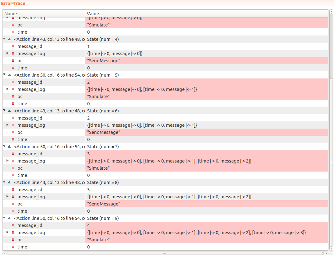
----------------------------- MODULE Throttling -----------------------------
EXTENDS Naturals, FiniteSets
CONSTANTS Window, Limit, MaxTime, Clients

(* --algorithm throttling
variables
    Time = 0,
    MessageLog = {};   

define
    GetTimeWindow(T) ==
        {X \in Nat : X <= T /\ X >= (T - Window)}
        
    SentMessages(Sender, TimeWindow) ==
        Cardinality({Message \in MessageLog: Message.Time \in TimeWindow /\ Message.Sender = Sender})
end define;   
 
macro SendMessage(Sender, Message)
begin
    MessageLog := MessageLog \union {[Time |-> Time, Message |-> Message, Sender |-> Sender]};
end macro;

process Server = 1
begin
    Simulate:
    while Time < MaxTime do
        Time := Time + 1;
    end while;
end process;

process Client \in Clients
variables MessageId = 0;
begin
    Simulate:
    while Time < MaxTime do
        if SentMessages(self, GetTimeWindow(Time)) < Limit then
            SendMessage(self, MessageId);
            MessageId := MessageId + 1;
        end if;
    end while;
end process;

    
end algorithm; *)

FrequencyInvariant ==
    \A C \in Clients: \A T \in 0..MaxTime: SentMessages(C, GetTimeWindow(T)) <= Limit

=============================================================================

Let’s try with a small model first: 2 clients, window of 2 seconds, modelled for 5 total seconds, with a limit of 3 seconds. 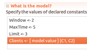Here client process names are defined as a set of model values. Model values are special values in TLA+ in that a value is only equal to itself and nothing else (C1 = C1, but C1 != C2, C1 != 5, C1 != FALSE, etc.), so it’s useful in avoiding mixing up with primitive types. Symmetry set can also be selected, as permutations in values of this set do not change the meaning: whether we have processes C1 and C2, or C2 and C1 - it doesn’t matter. Marking a set as a symmetry set, however, does allow TLC to reduce the search space and check specs faster.

When run with these values TLC doesn’t report any issues

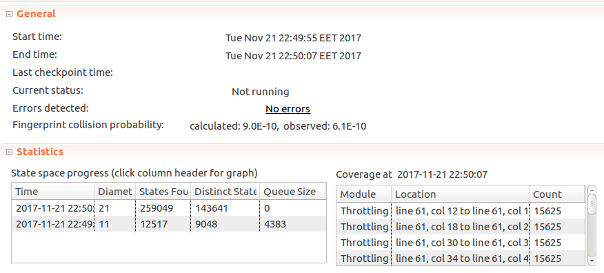
Looking good! But so far the spec only checks if the number of messages sent is at or below the limit. But zero messages sent is also under the limit! So if SendMessage altered to drop all messages:

macro SendMessage(Sender, Message)
begin
    MessageLog := {};
end macro;

And the model is rerun - TLC will get stuck on incrementing message IDs, but it should still pass. Not great! This fits the idea mentioned in the Amazon Paper, in which they suggest TLA+ forces one to think about what needs to go right. So what this model is still missing is at least to ensure if message can be sent - it is actually sent, not partially or incorrectly throttled.

But before going down that direction, there is a change to consider that would simplify the model and help resolve the infinite loop problem, thus helping demonstrate the message dropping issue more clearly.

Simplification

Hillel Wayne, author of the learntla.com, has recently helpfully suggested tracking number of messages sent using functions as opposed to tracking messages themselves, and counting them afterwards. It can be done because we don’t really care about message contents. Thanks for the tip!

To do that, Messages can be redefined as such:

variables
    Time = 0,
    SimulationTimes = 0..MaxTime,
    Messages = [C \in Clients |-> [T \in SimulationTimes |-> 0]];

Each client will have a function, which returns another function holding the number of messages a Client has sent at a particular Time. Then addressing a specific time of a particular client can be as simple as Messages[Client][Time].

The way time windows are calculated needs to change as well, as this time TLC was unable to use a finite integer set instead of Naturals set:

Attempted to enumerate { x \in S : p(x) } when S:
Nat
is not enumerable
While working on the initial state:
/\ Time = 0
/\ Messages = ( C1 :> (0 :> 0 @@ 1 :> 0 @@ 2 :> 0 @@ 3 :> 0 @@ 4 :> 0) @@
  C2 :> (0 :> 0 @@ 1 :> 0 @@ 2 :> 0 @@ 3 :> 0 @@ 4 :> 0) )
/\ pc = (C1 :> "Simulate" @@ C2 :> "Simulate" @@ 1 :> "Simulate_")
/\ SimulationTimes = 0..4

Here’s a response by Leslie Lamport detailing the issue a bit more. Rewritten GetTimeWindow as such:

GetTimeWindow(T) ==
    {X \in (T-Window)..T : X >= 0 /\ X <= T /\ X >= (T - Window)}

To count the number of messages, summing with reduce can be convenient. For that I borrowed SetSum operator from the snippet Hillel recommended, ending up with:

TotalSentMessages(Sender, TimeWindow) ==
    SetSum({Messages[Sender][T] : T \in TimeWindow})

The rest of the changes are trivial, so here’s the code:

----------------------------- MODULE ThrottlingSimplified -----------------------------
EXTENDS Naturals, FiniteSets, Sequences
CONSTANTS Window, Limit, MaxTime, Clients

(* --algorithm throttling
variables
    Time = 0,
    SimulationTimes = 0..MaxTime,
    Messages = [C \in Clients |-> [T \in SimulationTimes |-> 0]];

define
    GetTimeWindow(T) ==
        {X \in (T-Window)..T : X >= 0 /\ X <= T /\ X >= (T - Window)}
    
        
    Pick(Set) == CHOOSE s \in Set : TRUE

    RECURSIVE SetReduce(_, _, _)
    SetReduce(Op(_, _), set, value) == 
      IF set = {} THEN value
      ELSE 
        LET s == Pick(set)
        IN SetReduce(Op, set \ {s}, Op(s, value)) 
            
    SetSum(set) == 
      LET _op(a, b) == a + b
      IN SetReduce(_op, set, 0)
        
    TotalSentMessages(Sender, TimeWindow) ==
        SetSum({Messages[Sender][T] : T \in TimeWindow})
        
end define;   
 
macro SendMessage(Sender)
begin
    Messages[Sender][Time] := Messages[Sender][Time] + 1;
end macro;

process Server = 1
begin
    Simulate:
    while Time < MaxTime do
        Time := Time + 1;
    end while;
end process;

process Client \in Clients
begin
    Simulate:
    while Time < MaxTime do
        if TotalSentMessages(self, GetTimeWindow(Time)) < Limit then
            SendMessage(self);
        end if;
    end while;
end process;

    
end algorithm; *)

FrequencyInvariant ==
    \A C \in Clients: \A T \in SimulationTimes: TotalSentMessages(C, GetTimeWindow(T)) <= Limit

And if we run the model, it passes: 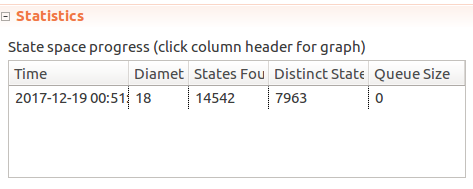But if + 1 is removed from the SendMessage macro, effectively quietly dropping all messages - the model still passes. Gah!

Ensuring messages do get sent

The idea to fix this issue is simple - track message sending attempts. The invariant would then check if enough messages have been sent.

To do so, a new variable MessagesAttempted is added:

MessagesAttempted = [C \in Clients |-> [T \in SimulationTimes |-> 0]];

And an operator to count the total number of attempts made during a window:

TotalAttemptedMessages(Sender, TimeWindow) ==
    SetSum({MessagesAttempted[Sender][T] : T \in TimeWindow})

Macro to mark the sending attempt:

macro MarkSendingAttempt(Sender)
begin
    MessagesAttempted[Sender][Time] := MessagesAttempted[Sender][Time] + 1;
end macro;

And updated the client process to mark sending attempts:

process Client \in Clients
begin
    Simulate:
    while Time < MaxTime do
        if TotalSentMessages(self, GetTimeWindow(Time)) < Limit then
            SendMessage(self);
            MarkSendingAttempt(self);
        end if;
    end while;
end process;

As for the invariant, there are two relevant cases: a) When there were fewer sending attempts than limit permits, all of them should be successfully accepted; b) When number of attempts is larger than the limit, number of messages successfully accepted should be at whatever Limit is set. Which could be written as such:

PermittedMessagesAcceptedInvariant ==
    \A C \in Clients:
        \A T \in SimulationTimes:
            \/ TotalAttemptedMessages(C, GetTimeWindow(T)) = TotalSentMessages(C, GetTimeWindow(T))
            \/ TotalAttemptedMessages(C, GetTimeWindow(T)) = Limit

Here’s the full code:

----------------------------- MODULE ThrottlingSimplified -----------------------------
EXTENDS Naturals, FiniteSets, Sequences
CONSTANTS Window, Limit, MaxTime, Clients

(* --algorithm throttling
variables
    Time = 0,
    SimulationTimes = 0..MaxTime,
    Messages = [C \in Clients |-> [T \in SimulationTimes |-> 0]],
    MessagesAttempted = [C \in Clients |-> [T \in SimulationTimes |-> 0]];

define
    GetTimeWindow(T) ==
        {X \in (T-Window)..T : X >= 0 /\ X <= T /\ X >= (T - Window)}
    
        
    Pick(Set) == CHOOSE s \in Set : TRUE

    RECURSIVE SetReduce(_, _, _)
    SetReduce(Op(_, _), set, value) == 
      IF set = {} THEN value
      ELSE 
        LET s == Pick(set)
        IN SetReduce(Op, set \ {s}, Op(s, value)) 
            
    SetSum(set) == 
      LET _op(a, b) == a + b
      IN SetReduce(_op, set, 0)
        
    TotalSentMessages(Sender, TimeWindow) ==
        SetSum({Messages[Sender][T] : T \in TimeWindow})
        
    TotalAttemptedMessages(Sender, TimeWindow) ==
        SetSum({MessagesAttempted[Sender][T] : T \in TimeWindow})
        
end define;   
 
macro SendMessage(Sender)
begin
    Messages[Sender][Time] := Messages[Sender][Time] + 1;
end macro;

macro MarkSendingAttempt(Sender)
begin
    MessagesAttempted[Sender][Time] := MessagesAttempted[Sender][Time] + 1;
end macro;

process Server = 1
begin
    Simulate:
    while Time < MaxTime do
        Time := Time + 1;
    end while;
end process;

process Client \in Clients
begin
    Simulate:
    while Time < MaxTime do
        if TotalSentMessages(self, GetTimeWindow(Time)) < Limit then
            SendMessage(self);
            MarkSendingAttempt(self);
        end if;
    end while;
end process;

    
end algorithm; *)

FrequencyInvariant ==
    \A C \in Clients: \A T \in SimulationTimes: TotalSentMessages(C, GetTimeWindow(T)) <= Limit
    
PermittedMessagesAcceptedInvariant ==
    \A C \in Clients:
        \A T \in SimulationTimes:
            \/ TotalAttemptedMessages(C, GetTimeWindow(T)) = TotalSentMessages(C, GetTimeWindow(T))
            \/ TotalAttemptedMessages(C, GetTimeWindow(T)) = Limit

If messages are successfully accepted, the model passes. However, if SendMessage is purposefully broken again by commenting out the incrementation, the model fails:

Invariant PermittedMessagesAcceptedInvariant is violated.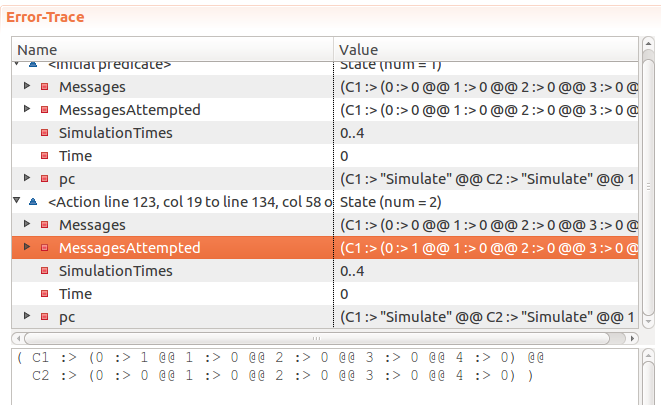

Which is great, as this is exactly what we wanted to achieve.

Last time we briefly looked over resources for learning TLA+ and PlusCal, as well as wrote a basic spec to prove equivalence of a few logic formulas. In this post I thought it would be interesting to write a spec for a more common scenario.

The idea

This is inspired by the issue we had with MailPoet 2. An attacker was able to successfully continuously sign up users, the users would get sent a subscription confirmation email with each subscription, that way some email addresses were effectively bombed with emails. Let’s try to model and explore this situation.

In the actual system we have the client, server, emails being sent out, network connections… Lots of details, most of them we can probably ignore safely and still model the system sufficiently.

Sending messages without any rate-limiting

Let’s start with the initial situation: we want to allow TLC to send arbitrary “Messages” (actual content, metadata is irrelevant here) over time, and we want to put some limit on how many messages can be sent out over some period of time.

For a start we’ll model just a single sender, storing messages in a set as a log, noting their contents and time when they were sent. Contents would be irrelevant, but in this case it helps humans interpret the situation. We’ll allow TLC to keep sending an arbitrary number of messages one by one, and then increment the time. That way we allow our model to “send 60 messages in one second”.

Finally, we add an invariant to make sure that the number of messages sent in one second does not go over the limit. Here’s the code:

----------------------------- MODULE Throttling -----------------------------
EXTENDS Naturals, FiniteSets
CONSTANTS Window, Limit, MaxTime

(* --algorithm throttling
variables
    Time = 0,
    MessageId = 0,
    MessageLog = {};

macro SendMessage(Message)
begin
    MessageLog := MessageLog \union {[Time |-> Time, Message |-> Message]};
end macro;

begin
    Simulate:
    while Time < MaxTime do
        either
            SendMessage:
                SendMessage(MessageId);
                MessageId := MessageId + 1;
        or
            TimeStep:
                Time := Time + 1;
        end either;
    end while;
end algorithm; *)

FrequencyInvariant ==
    \A T \in 0..MaxTime: (Cardinality({Message \in MessageLog: Message["Time"] = T}) <= Limit)

The individual log in MessageLog is a record with 2 keys: Time and Message, and the MessageLog itself is a set. The FrequencyInvariant invariant checks that during every second of our simulation the number of messages sent does not exceed our Limit.

We’ll use these constant values for our initial runs:

Window <- 3
MaxTime <- 5
Limit <- 3

If we translate the PlusCal code to TLA+ (with Ctrl+T in Toolbox) and run the model with TLC, as we expected - it quickly finds an error:

Since we did not perform any throttling and instead allowed TLC to “send” an arbitrary number of messages - TLC sent 4 messages before the invariant failed.

Time based throttling

As the next step let’s make use of the Window constant and alter SendMessage() macro to accept messages only if doing so does not exceed our Limit.

First of all, given a Time, we want to grab a set of times falling within our window. So if the current Time = 5, and our Window = 2, we want it to return {3, 4, 5}:

define
  GetTimeWindow(T) ==
      {X \in Nat : X <= T /\ X >= (T - Window)}
\* ...

Next, we want to define a way to count the number of messages sent over a set of specific times. So if our time window is {3, 4, 5, 6}, we count the total number of messages sent at Time = 3, Time = 4, …, Time = 6:

\* ...
    SentMessages(TimeWindow) ==
            Cardinality({Message \in MessageLog: Message.Time \in TimeWindow})
end define;

Then we can write a ThrottledSendMessage variant of the SendMessage macro:

macro ThrottledSendMessage(Message)
begin
    if SentMessages(GetTimeWindow(Time)) < Limit then
        SendMessage(Message);
    end if;
end macro;

Here we silently drop the overflow messages, “sending” only what’s within the limit. At this point this is the code we have:

----------------------------- MODULE Throttling -----------------------------
EXTENDS Naturals, FiniteSets
CONSTANTS Window, Limit, MaxTime

(* --algorithm throttling
variables
    Time = 0,
    MessageId = 0,
    MessageLog = {};   

define
    GetTimeWindow(T) ==
        {X \in Nat : X <= T /\ X >= (T - Window)}
        
    SentMessages(TimeWindow) ==
        Cardinality({Message \in MessageLog: Message.Time \in TimeWindow})
end define;   
 
macro SendMessage(Message)
begin
    MessageLog := MessageLog \union {[Time |-> Time, Message |-> Message]};
end macro;

macro ThrottledSendMessage(Message)
begin   
    if SentMessages(GetTimeWindow(Time)) < Limit then
        SendMessage(Message);
    end if;
end macro;
     
begin
    Simulate:
    while Time < MaxTime do
        either
            SendMessage:
                ThrottledSendMessage(MessageId);
                MessageId := MessageId + 1;
        or
            TimeStep:
                Time := Time + 1;
        end either;
    end while;    
end algorithm; *)

FrequencyInvariant ==
    \A T \in 0..MaxTime: (Cardinality({Message \in MessageLog: Message["Time"] = T}) <= Limit)

=============================================================================

At this point we can run our model:

And hmm… After 10-20 minutes of checking TLC does not finish, the number of distinct states keeps going up. I even tried reducing our constants to Window <- 2, MaxTime <- 3, Limit <- 3. As TLC started climbing over 2GB of memory used I cancelled the process. Now what?

Assuming that the process could never terminate, what could cause that? We tried to limit our “simulation” to MaxTime <- 3, time keeps moving on, number of messages “sent” is capped by Limit. But looking back at the SendMessage label, ThrottledSendMessage() gets called and it’s result isn’t considered. But regardless of whether or not a message has been sent, MessageId always keeps going up, and each such new state could mean TLC needs to keep going. So that’s the hypothesis.

Let’s try capping that by moving MessageId := MessageId + 1; from SendMessage label to ThrottledSendMessage macro, and perform it only if the message is successfully sent. Now if we rerun the model: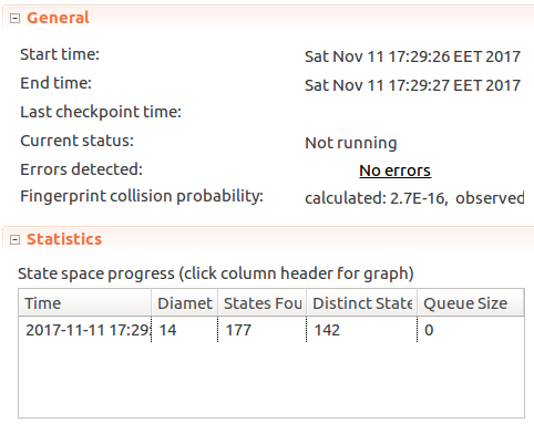

We can see that TLC has found no errors, TLC found 142 distinct states and the number of messages sent at any single Time value hasn’t exceeded Limit <- 3. Great!

Next let’s strengthen the FrequencyInvariant. Right now it checks whether the number of messages sent at ONE SPECIFIC VALUE OF Time does not exceed the Limit. But we want to ensure that the same holds for the whole Window of time values:

FrequencyInvariant ==
    \A T \in 0..MaxTime: SentMessages(GetTimeWindow(T)) <= Limit

And because the spec already had implemented time-window based rate limiting - the number of states checked stayed the same:

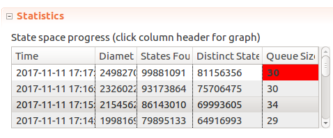
At this point running TLC with smaller model sizes helped build confidence in the model. But will it hold if we crank up constants to say… Window <- 5, MaxTime <- 30, Limit <- 10? Unfortunately in an hour of running the model the number of distinct states and queue size just kept going up at a consistent pace, so after it consumed over 1gb of memory it had to be terminated.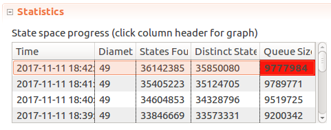

I think Limit being high creates quite a few states, as you can spread out 10 messages over 5 distinct times in 5^10 ways. Spread that out over 30-5+1=26 possible windows, bringing us into hundreds of millions of possible states. The number of states quickly goes up even in this fairly simple case! It took my laptop ~10 minutes to explore ~13 million states reached with Window <- 5, MaxTime <- 15, Limit < 5 configuration: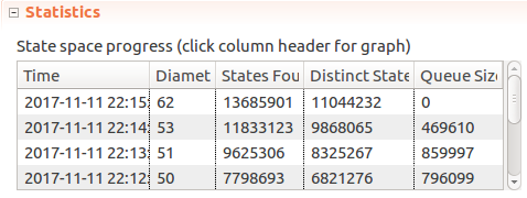

For the sake of the example that’s probably sufficient. I don’t see any point in checking larger models in this case, but on a faster computer, or on a distributed set of servers it could be checked much faster. Yes - TLC does work in a distributed mode, which could be an interesting feature to play around in itself.

When you hear about formal methods in the context of software development, what do you picture in your mind? I would imagine a time consuming and possibly tedious process used in building mission-critical software, e.g. for a pacemaker or a space probe.

It may be something briefly visited during Computer Science courses at a college or university, quickly running through a few trivial examples. I have never actually had a chance to look into them before, so after reading the “loudly” titled “The Coming Software Apocalypse” in The Atlantic (interesting article by the way), it seemed intriguing.

Furthermore, interest has been elevated furthermore by the fact that Amazon Web Services team has had good success in using formal methods in their day to day work and they are continuing to push its adoption. (Use of Formal Methods at Amazon Web Services)

So the goal here is to learn enough about formal methods to be able to use them in at least one case on my own, whether at work or on a pet project. And just because there are a few books about TLA+ - that will be the focus of this experiment.

Why?

TLA+ is built to model algorithms and systems, to make sure they work as expected and catch any bugs lurking in them. It can be very helpful in finding subtle bugs in non-trivial algorithms or systems we create. When you write a specification, TLA+ Toolbox comes with a TLC Model checker that will check your specification and try to find issues in it. E.g. in one of the examples a bug TLC found took about 30 steps to reproduce. It also provides tools to explore certain properties of your system in question, e.g. what the system is allowed to do, or what the system eventually needs to do. This improves our confidence in systems we build.

With TLA+ we are working with a model of a system, which can work with and against us. With a model we can iterate faster, glossing over irrelevant details, exploring our ideas before we build out the final systems. But because we work with a model, we have to take great care in describing the model as to not gloss over critical behavior-altering details.

The other benefit we get is better understanding of systems we build, how they work and how they may fail. In order to write a spec it forces you to think about what needs to go right. To quote the AWS paper above, “we have found this rigorous “what needs to go right?” approach to be significantly less error prone than the ad hoc “what might go wrong?” approach.”

Learning about TLA+

To start with, Leslie Lamport produces a TLA+ Video Course. They will very clearly explain how TLA+ works, how to set up the Toolbox and get it running, run and write a few specifications as well, including parts of widely used algorithms, such as Paxos Commit (video version, paper).

Once up and running, mr. Lamport’s “Specifying systems” book provides an even more detailed look of TLA+. The book is comprehensive and can be a tough read, however it comprises of multiple parts and the first part “contains all that most engineers need to know about writing specifications” (83 pages).

And if you have checked out any of the specifications shared in the book and videos above, you may find that the way specifications are written is slightly different compared to the day-to-day programming languages one may use. Luckily, the Amazon paper mentions PlusCal, which is an accompanying language to TLA+ and feels more like a regular C-style programming language. They also report some engineers being more comfortable and productive with PlusCal, but still requiring extra flexibility provided by TLA+. You can learn more about PlusCal in Hillel Wayne’s online book Learning TLA.

Exploring tautologies

A tautology is defined as “[…] a formula which is “always true” — that is, it is true for every assignment of truth values to its simple components. You can think of a tautology as a rule of logic.” (ref). And in formal logic there are formulas which are equivalent, e.g. A -> B (A implies B) is equivalent to ~A \/ B (not A or B). So as a very basic starting point we can prove that with TLA+.

---------------------------- MODULE Tautologies ----------------------------
VARIABLES P, Q

F1(A, B) == A => B
F2(A, B) == ~A \/ B

FormulasEquivalent == F1(P, Q) <=> F2(P, Q)

Init ==
    /\ P \in BOOLEAN
    /\ Q \in BOOLEAN

Next ==
    /\ P' \in BOOLEAN
    /\ Q' \in BOOLEAN

Spec ==
    Init /\ [][Next]_<<P, Q>>
=============================================================================

The idea here is fairly simple: Let TLC pick arbitrary set of 2 boolean values, and we make sure that whatever those values are - results of F1 and F2 are always equivalent.

We declare 2 variables in our spec: P and Q. In the Init method we declare that both variables have some value from BOOLEAN set (which is equal to {TRUE, FALSE}). We don’t have to specify which particular values - TLC will pick them for us. Next is our loop step to mutate the values of P and Q. P' designates what the value of P will be after Next is executed. Again - we allow it to be any value from BOOLEAN set. This is important, because if we didn’t specify how exactly to mutate the value (or not change it) - TLC is free to pick an arbitrary value for it: NULL, "somestring", set {2, 5, 13}, etc. So up to this point we only allowed TLC to pick values of P and Q. They could be P = FALSE, Q = FALSE, P = FALSE, Q = TRUE, P = TRUE, Q = FALSE, P = TRUE, Q = TRUE.

We check our condition by configuring TLC to check if our invariant FormulasEquivalent holds. An invariant is a property that has to hold as the data mutates. In our case it’s “whatever P and Q values are, results of F1(P, Q) and F2(P, Q) should be equivalent”.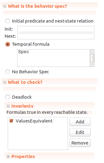

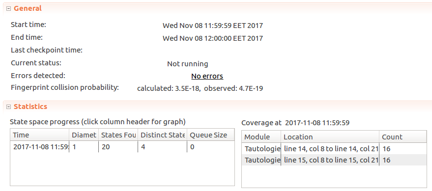
Once we run TLC, it reports that there were 4 distinct states (as we expected), and that there are no errors - our model worked as we expected.

Now, if we intentionally make a mistake and declare F2 as F2(A, B) == A \/ B by replacing ~A with A (removing negation), we can rerun the model and see what TLC finds: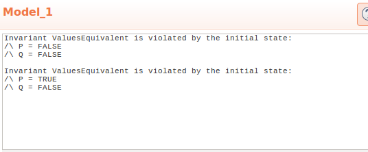

We see that TLA found two states where our invariant does not hold:

Invariant FormulasEquivalent is violated by the initial state:
/\ P = FALSE
/\ Q = FALSE

Invariant FormulasEquivalent is violated by the initial state:
/\ P = TRUE
/\ Q = FALSE

Which is exactly what we expected. Similarly we can check equivalence for ~(A /\ B) <=> (~A \/ ~B), P <=> (P \/ P), (P => Q) <=> (~Q => ~P), etc. Useful? Not very, but it gets us writing and checking some basic specs.

Closing thoughts

After running through the tutorial videos, first part of the “Specifying systems” book and “Learn TLA+” book I thought I had the grasp of it, but the air quickly ran out once I turned to attempting write specifications without external guidance. Perhaps specifying a sorting algorithm or solving a magic square was too much to quick and more practice is needed with simpler specifications. Finding an interesting yet achievable algorithm to specify is proving to be a challenge. So this part stops here with only the first trivial spec for proving equivalent logic formulas, and in the next part it may be interesting to try specifying a basic rate limiting algorithm.

In the meantime, running through TLA+ examples on Github helped better understand the types of algorithms TLA+ can specify and the way more complex specifications are written.

Recently I wanted to figure out a bit more about how popular WordPress plugins are used. Helpfully, WordPress plugin repository does provide a JSON API endpoint for fetching download statistics of any plugin in the plugin repository, e.g.:

https://api.wordpress.org/stats/plugin/1.0/downloads.php?slug=akismet&limit=365

It is used for plotting the stats on plugin pages, and it works for my purpose as well.

There are two things I wanted to know from these stats: 1) How many downloads happen on average each day of the week; 2) How many total downloads happen in a week

First I started by manually importing the data into LibreOffice Calc and calculating the moving weekly sums and moving 7d averages myself (for each daily downloads cell sum over last 7 ones, and average over last 7 ones).

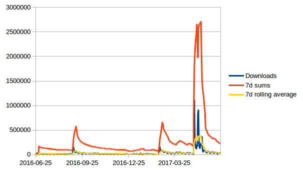
For a quick plot it worked, but was not very convenient to update if you would like to take a look at multiple plugins every so often. So this was my excuse to play around with Pandas and Matplotlib to build something a bit more convenient in Python.

Setup

To begin we’ll use several libraries:

• Requests to download the JSON stats;
• Pandas for data manipulation and to run our extra calculations;
• Matplotlib to plot the results.

As usual, we start by creating a virtual environment. For this I used Python 3:

virtualenv -p python3 venv
source venv/bin/activate

And installed the dependencies in our virtual environment:

pip install requests matplotlib pandas

We start with the initial dependencies and download the stats from WP plugin repo:

import pandas as pd
import json, time, requests
import matplotlib.pyplot as plt
from matplotlib import style

url = 'https://api.wordpress.org/stats/plugin/1.0/downloads.php?slug=akismet&limit=365'
r = requests.get(url)
data = r.json()

data now contains a dict with dates for keys, and number of downloads for values. DataFrame expects a list-like object for data parameter, so we will need to reshape the data first from dict to a list of dicts. While we’re at it, we’ll convert date strings into date objects:

data = [
    { 'timestamp': pd.to_datetime(timestamp, utc=False), 'downloads': int(downloads) }
    for (timestamp, downloads) in data.items()]
data = sorted(data, key=lambda item: item['timestamp'])

At this point we have converted the initial stats dictionary:

{'2017-03-21': '36723', '2016-08-17': '18061', '2016-06-26': '17821', '2016-09-14': '52539', ...}

Into a list of dictionaries:

[{'timestamp': Timestamp('2016-06-25 00:00:00'), 'downloads': 18493}, ...]

However, if we pass the resulting list into a Pandas DataFrame, we will see that it is indexed by row number, instead of by date:

>>> pd.DataFrame(data)
     downloads  timestamp
0        18493 2016-06-25
1        17821 2016-06-26
2        29163 2016-06-27
3        28918 2016-06-28
4        27276 2016-06-29
...

To fix that, we reindex the resulting DataFrame on timestamp column:

df = pd.DataFrame(data)
df = df.set_index('timestamp')

And get:

>>> df
            downloads
timestamp            
2016-06-25      18493
2016-06-26      17821
2016-06-27      29163
2016-06-28      28918
...

Now that we have our raw data, let’s calculate the 7 day average. DataFrame.rolling() works nicely for this:

weekly_average = df.rolling(window=7).mean()

The way it works is it takes a number of sequential data points (in our case - 7 days) and performs an aggregate function over it (in our case it’s mean()) to create a new DataFrame:

>>> weekly_average
               downloads
timestamp               
2016-06-25           NaN
2016-06-26           NaN
2016-06-27           NaN
2016-06-28           NaN
2016-06-29           NaN
2016-06-30           NaN
2016-07-01  24177.857143
2016-07-02  23649.857143
2016-07-03  23186.857143
2016-07-04  22186.428571
...

We can use the same approach to calculate weekly sums:

>>> weekly_sum = df.rolling(window=7).sum()
            downloads
timestamp            
2016-06-25        NaN
2016-06-26        NaN
2016-06-27        NaN
2016-06-28        NaN
2016-06-29        NaN
2016-06-30        NaN
2016-07-01   169245.0
2016-07-02   165549.0
2016-07-03   162308.0
...

Now onto plotting. We want to display all 3 series (raw downloads, weekly averages and weekly sums) on a single plot, to do that we create a subplot:

# Setting the style is optional
style.use('ggplot')
fig, ax = plt.subplots()

fig is the figure, and ax is the axis.

We could call the df.plot() command and it would work, but before we do that let’s set up more presentable column names for the legend:

df.columns = ['Daily downloads']
weekly_average.columns = ['Weekly average']
weekly_sum.columns = ['Weekly sum']

ax.set_xlabel('Time')
ax.set_ylabel('Downloads')
ax.legend(loc='best')

And lastly we plot the data:

df.plot(ax=ax, label="Daily downloads", legend=True, style='r-', title="Downloads")
weekly_average.plot(ax=ax, label="7 day average", legend=True, style='b-')
weekly_sum.plot(ax=ax, label="7 day sum", legend=True, style='r--')
plt.show()

For line styles, r- refers to a solid red line, r-- is a dashed red line, and b- is a solid blue line. You can refer to lines_styles.py example and lines styles reference for more details on styling.

Results

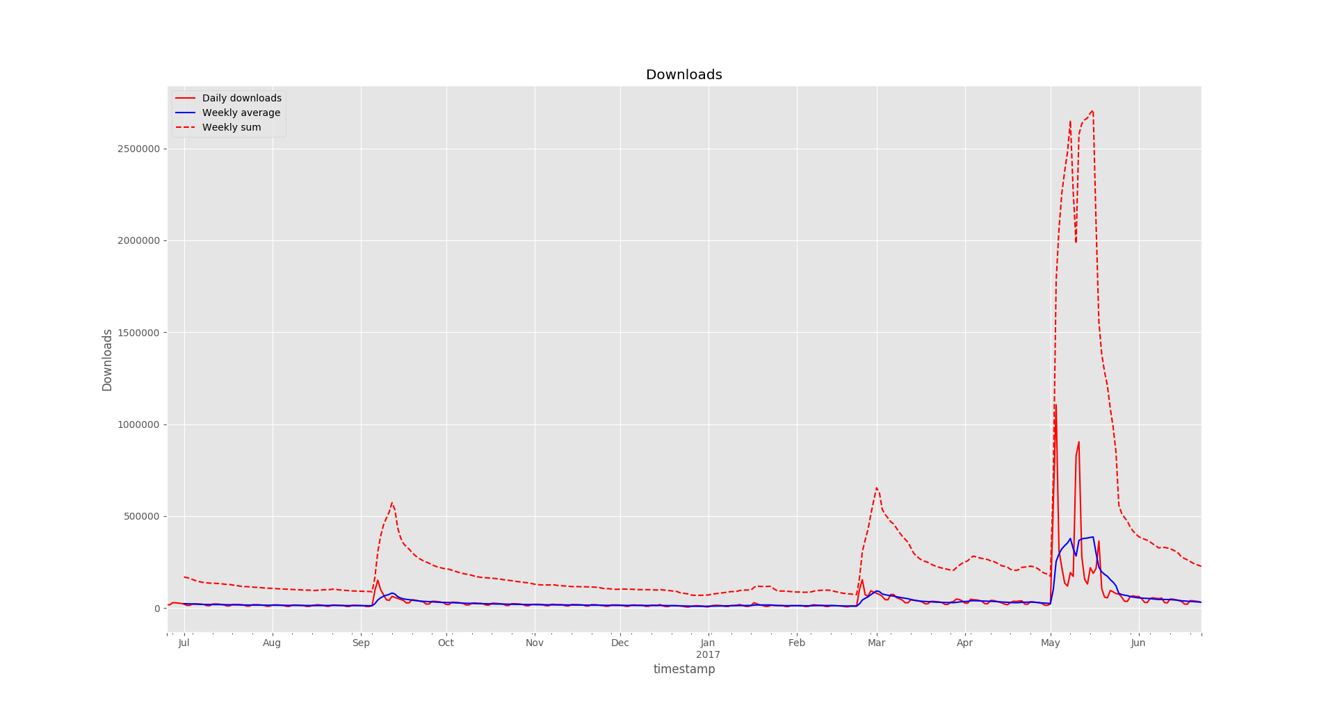
Visually perhaps it looks somewhat similar to the LibreOffice Calc variant, but with some extra effort we could generate graphs for a much larger number of plugins, add extra data or metrics, generate image files. And now we can use Matplotlib tools to zoom in and out of different sections while looking at specific details in the plot.

The final code looked like this:

import pandas as pd
import json, time, requests
import matplotlib.pyplot as plt
from matplotlib import style

url = 'https://api.wordpress.org/stats/plugin/1.0/downloads.php?slug=akismet&limit=365'
r = requests.get(url)
data = r.json()
data = [
    { 'timestamp': pd.to_datetime(timestamp, utc=False), 'downloads': int(downloads) }
    for (timestamp, downloads) in data.items()]
data = sorted(data, key=lambda item: item['timestamp'])

df = pd.DataFrame(data)
df = df.set_index('timestamp')

weekly_average = df.rolling(window=7).mean()
weekly_sum = df.rolling(window=7).sum()

style.use('ggplot')
fig, ax = plt.subplots()

df.columns = ['Daily downloads']
weekly_average.columns = ['Weekly average']
weekly_sum.columns = ['Weekly sum']

ax.set_xlabel('Time')
ax.set_ylabel('Downloads')
ax.legend(loc='best')

df.plot(ax=ax, label="Daily downloads", legend=True, style='r-', title="Downloads")
weekly_average.plot(ax=ax, label="7 day average", legend=True, style='b-')
weekly_sum.plot(ax=ax, label="7 day sum", legend=True, style='r--')
plt.show()

I really enjoy trading as my primary activity in the online game Eve Online - it’s fun seeing your wallet grow. People call it “spreadsheet simulator in space” for a reason, it’s especially relevant if you’re into trading or industry - you have to calculate your profits!

It can be quite difficult to gauge profitability of a particular trade - you have to consider the margin, market movement and competition. With thousands of tradable items and thousands of markets - it can be challenging to find profitable items, which is why people build various tools to do that automatically. Estimating competition can be difficult. Unless you’re actively trading in an item - you often don’t know if someone will actively outbid you every minute, or if your order will stay at the top for days.

And this is what this mini project is about. I’ll focus more on technical details, since this is not a gaming blog and the game is just an outlet for the project.

What is trading and how it works, problem area

If you’re familiar with real life stock trading, this will probably sound familiar. But if you’re not, here’s how trading works in a nutshell.

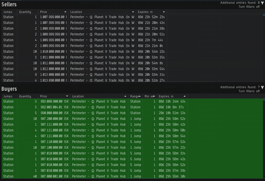
There are buy and sell orders. If you want to sell something, you can create a sell order for that item by specifying a price, and it will be created on the market. If someone wants to buy the item from you, they will have to pay your quoted price in exchange for the item. Sell orders are always fulfilled from the lowest price to the highest price, meaning that if there are two orders for 1$ and 2$ and someone wants to buy an item, the 1$ order will always be fulfilled first regardless of whether the buyer is willing to pay 2$ for it. Respectively, if you want to buy something, you can put up a buy order for a specific price and number of items (e.g. “I am willing to pay X$ each for 20 items”). If someone chooses to sell you an item, an exchange will be made, the seller will get your money, and you will get the item. Buy orders are fulfilled from the highest price to the lowest price. So higher-priced orders will be fulfilled first, hence the goal of keeping your orders on top.

You want to keep your orders on top to sell (or buy) your items fastest. However, if there are 10 other people trying to do the same thing at the same time - clearly that will be difficult. And in fierce markets your orders can be outbid in under 10 seconds!

Also, it’s worth mentioning that in Eve Online you cannot further update an order for 5 minutes after an order is created or last updated

So, knowing the times when your competition is active can be very helpful. Then you can come in just after they’re gone and get back to the top order for much longer, or spend less effort doing that.

Concept and technical setup

Going into this mini project, there is one main question I want an answer to: at what time(s) of day traders tend to update their orders. Optionally, it would be good to know how often they update their orders, or many items are sold at specific times of day.

The idea is to passively watch the market by taking snapshots of active orders, noting their IDs, prices and timestamps of latest update. Since orders can be updated only after 5 minutes, and the endpoint is cached for 5 minutes, it likely is a good enough approximation to take snapshots every 5 minutes. Once we have that information, we can use the database to group order updates into intervals and simply count the number of rows in each interval to get the number of updated orders.

I’ve learned about InfluxDB (a time series database) at work, and since then I’ve been meaning to find a personal project to use it on. Their Why time series data? page suggests several different use cases, such as tracking financial markets, sensor data or infrastructure data, which seems like a good fit for my problem.

I set up InfluxDB using the Getting Started guide, and used influxdb-python package for interacting with the DB.

Eve Online is special here, because they very actively expose game data via public APIs for 3rd party developers. So we can use their helpfully provided new ESI JSON API to query market data.

Implementation

We can fetch the market data from the JSON endpoint by making an HTTP request (Market > Orders endpoint docs). This can be done with requests library:

import requests

def get_item_orders(item_id, region_id, page=1, order_type='all'):
    esi_root = 'https://esi.tech.ccp.is/latest'
    url = '%s/markets/%d/orders/?type_id=%d&order_type=%s&page=%d&datasource=tranquility' % (
        esi_root,
        region_id,
        item_id,
        order_type,
        page
    )
    r = requests.get(url)
    response = r.json()
    if 'error' in response:
        raise Exception('Failed to get item orders', item_id, region_id, response)
    else:
        return response

Which returns a response in this format:

[{
  u'volume_remain': 4,
  u'type_id': 40520,
  u'order_id': 4696910017,
  u'issued': u'2016-12-01T10:20:35Z',
  u'price': 787000000.0,
  u'min_volume': 1,
  u'is_buy_order': False,
  u'range': u'region',
  u'duration': 90,
  u'volume_total': 4,
  u'location_id': 61000990
}, ...]

Here we mostly care about issued, type_id, location, order_id, is_buy_order, price and volume_remain. issued denotes when the order was created or last updated, type_id denotes which item is being sold/bought.

Storing data in InfluxDB was straightforward with influxdb-python library:

from influxdb import InfluxDBClient

db = InfluxDBClient('localhost', 8086, 'root', 'root', 'market')

def fetch_orders():
    item_type_id = 40520
    region_id = 10000046

    try:
        orders = get_item_orders(item_type_id, region_id)
    except Exception as ex:
        print 'Failed to fetch orders'
        print ex
        return

    measurements = []
    for order in orders:
        measurements.append({
            'measurement': 'trade_history',
            'tags': {
                'region_id': region_id,
                'location_id': order['location_id'],
                'type_id': order['type_id'],
                'order_id': order['order_id'],
                'order_type': 'buy' if order['is_buy_order'] else 'sell'
            },
            'time': order['issued'],
            'fields': {
                'price': order['price'],
                'volume_remain': order['volume_remain'],
            }
        })

    db.write_points(measurements)
    print '[%s] %d orders fetched' % (datetime.datetime.now(), len(orders))

Here we simply iterate over a list of order objects, and out of them construct a list of measurement points. region_id, location_id, type_id, order_id and order_type don’t change even when an order is updated. Here an important point is to use the issued timestamp for the measurement time. That way we can accurately track when an order has been updated, and successive data fetches won’t duplicate the data.

If we run the code and check results in InfluxDB, we can see what we have:

> SELECT * FROM "trade_history" LIMIT 10;
name: trade_history
-------------------
time                    location_id     order_id        order_type      price                   region_id       type_id volume_remain
2016-10-30T20:37:10Z    61000647        4597357707      buy             5.6300000052e+08        10000046        40520   4
2016-11-21T07:07:57Z    61000990        4633264567      sell            7.8800000001e+08        10000046        40520   8
2016-12-01T10:20:35Z    61000990        4696910017      sell            7.87e+08                10000046        40520   4
2016-12-03T10:14:26Z    61000647        4699246159      sell            7.8300000052e+08        10000046        40520   2
2016-12-19T23:59:49Z    61000896        4657031429      buy             881                     10000046        40520   10
2016-12-28T19:58:22Z    61000647        4697110149      buy             4.13e+08                10000046        40520   1
2016-12-28T22:55:09Z    61000990        4667323418      buy             4.130000001e+08         10000046        40520   2
2016-12-31T08:13:49Z    61000990        4733297519      sell            7.19999998e+08          10000046        40520   5
2016-12-31T08:30:24Z    61000990        4733307476      sell            7.19999997e+08          10000046        40520   5
2016-12-31T08:39:25Z    61000990        4729427547      sell            7.1999999699e+08        10000046        40520   4

And lastly, to run this function every 5 minutes, schedule library comes in quite handy:

import schedule

schedule.every(5).minutes.do(fetch_orders)
while True:
  schedule.run_pending()
  time.sleep(1)

And now we have a Python script which will fetch outstanding market orders every 5 minutes and will log data to InfluxDB. At this point I left it running for several hours to gather some more data.

The last step is to query the data from InfluxDB. It was very important to use issued order value as the timestamp for storing data in InfluxDB, because it changes each time an order is updated. When an order is updated, it retains most of its data unchanged, however the issued and price fields will change. Hence, if an order was not updated at the time of checking, it will not be included in the data groups of that particular time chunk. That allows us to write this query:

SELECT COUNT("volume_remain") FROM "trade_history" WHERE "order_type"='sell' AND type_id='40520' AND time > now() - 7h GROUP BY time(30m)

Which yields this result:

> SELECT COUNT("volume_remain") FROM "trade_history" WHERE "order_type"='sell' AND type_id='40520' AND time > now() - 7h GROUP BY time(30m)
name: trade_history
-------------------
time                    count
2016-12-31T12:00:00Z    4
2016-12-31T12:30:00Z    0
2016-12-31T13:00:00Z    3
2016-12-31T13:30:00Z    0
2016-12-31T14:00:00Z    5
2016-12-31T14:30:00Z    7
2016-12-31T15:00:00Z    6
2016-12-31T15:30:00Z    11
2016-12-31T16:00:00Z    8
2016-12-31T16:30:00Z    9
2016-12-31T17:00:00Z    0
2016-12-31T17:30:00Z    6
2016-12-31T18:00:00Z    6
2016-12-31T18:30:00Z    2
2016-12-31T19:00:00Z    0

It’s not very important for this excercise, but we can take one more step and graph the results:

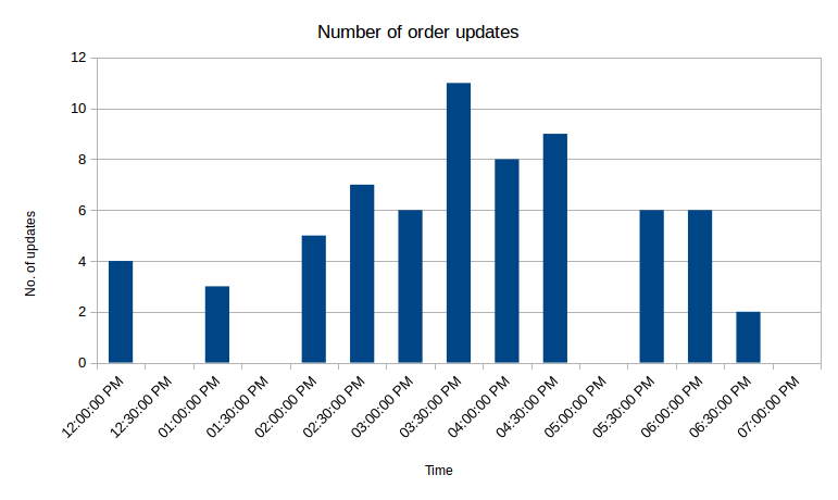
Graphing the price was not nearly as interesting, as compared to the price, differences are at most of several thousand ISK, which doesn’t show up well on the graph.

Gotchas

At first I was struggling to get a WHERE clause to work when writing InfluxDB queries: whenever I used WHERE - my queries returned no results. It turns out that InfluxQL requires using single quotes for denoting values, so this query will work:

SELECT * FROM trade_history WHERE "order_type"='sell'

While this will not:

SELECT * FROM trade_history WHERE "order_type"="sell"

Final thoughts

So in the 7 hours the script was running, there were over 50 order updates, and there were up to 11 updates in 30 minutes, which is very competetive. If you wanted your orders to stay on top, you’d have to trade quite actively in this particular location. But this is a great result. Just by glancing at outstanding orders it can be easy to be mistaken at how competetive competitors will be, but seeing longer term data paints a different picture. It would be useful to collect several days worth of data for several different items to evaluate the situation better, but this is already a good starting point.

It would be quite interesting to get access to raw data of actual real life stock exchanges and run the same script on the data. Some Bitcoin exchanges actually publicly display these orders as well, e.g. Real Time Bitcoin Ticker can be interesting to watch.